Signals and Systems · Continuous-time sinusoidal and exponential signals

#12 Amplitude, frequency, phase and exponential envelopes

Read sinusoidal amplitude, period and phase shift, distinguish one-sided from two-sided exponential decay, and describe a damped oscillation with its envelope.

Question

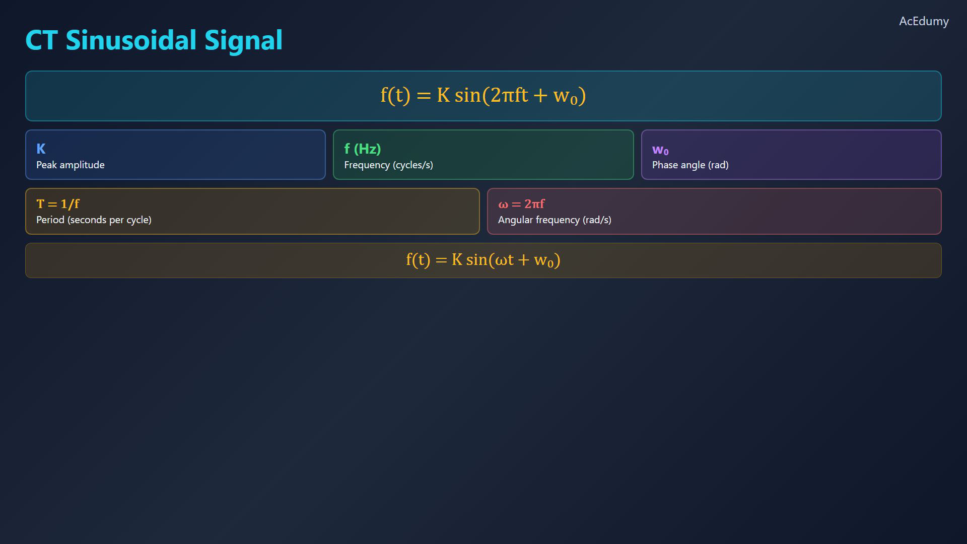
Original final-video graph or reference card for sinusoidal and exponential signals. — Original-video reference. In the sinusoid graph the purple arrow marks the time advance associated with phase. In the exponential comparison the far-left green segment is capped at 7.5 by the plotting code; the actual exponential continues growing as time tends to negative infinity. The damped graph is captured before the later erroneous peak markers appear; its formula is developed in the notebook lines.

Use positive peak amplitude K, frequency f and decay rate a for the examples in this lesson. The signal f(t) and the scalar frequency f use the source notation; omega is angular frequency and w_0 is phase in radians. The time shift is negative phase divided by omega. Choose u(0)=1 for the one-sided exponential. The two-sided exponential grows as t tends to negative infinity and decays as t increases. The comparison plot uses K=2 and a=0.5 and caps the far-left drawing at 7.5; evaluate the equation for actual values. The damped graph uses K=2,a=0.35,omega=4π,w_0=0. Its extrema lie inside the exponential envelope and its zero crossings are distinct from its peaks. Consecutive positive peaks shrink by a factor exp(−aT); the damped signal itself is not periodic. Physical examples refer to underdamped free or transient responses; external forcing can add a steady component.

Written solution and narration transcript(shows the full solution)

Below are all the lines written in the notebook together with the full narration transcript.

1. Define a continuous-time sinusoid
Original-video reference. In the sinusoid graph the purple arrow marks the time advance associated with phase. In the exponential comparison the far-left green segment is capped at 7.5 by the plotting code; the actual exponential continues growing as time tends to negative infinity. The damped graph is captured before the later erroneous peak markers appear; its formula is developed in the notebook lines.
Three signal types: sinusoidal, exponential and damped sinusoidal.
Sinusoidal signal:
$\displaystyle f\left(t\right)=K \sin \left(2\pi f t+w_{0}\right)$
With positive K, the maximum value is K and the minimum is negative K.
Frequency counts complete cycles per second and is measured in hertz.
Period for positive frequency:
$\displaystyle T=\frac{1}{f}$
The phase in radians determines a horizontal time shift.
Angular frequency in radians per second:
$\displaystyle \omega =2\pi f$
Equivalent signal:
$\displaystyle f\left(t\right)=K \sin \left(\omega t+w_{0}\right)$
Narration transcript
Today we introduce three important continuous-time signal types, starting with the sinusoidal signal. The general form is f of t equals K times sine of two pi f t plus w zero. Here K is the peak amplitude — the maximum value the signal reaches. The parameter f is the frequency in hertz, which tells us how many complete cycles occur per second. The period T equals one over f, giving the duration of one cycle. The phase angle w zero shifts the signal along the time axis. We commonly define the angular frequency omega as two pi f, measured in radians per second. This gives us the equivalent form: f of t equals K sine of omega t plus w zero.
2. Read amplitude, period and phase shift
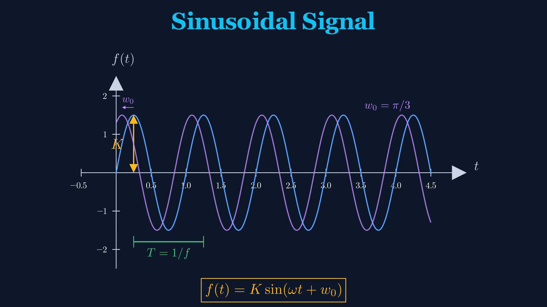
Original-video reference. In the sinusoid graph the purple arrow marks the time advance associated with phase. In the exponential comparison the far-left green segment is capped at 7.5 by the plotting code; the actual exponential continues growing as time tends to negative infinity. The damped graph is captured before the later erroneous peak markers appear; its formula is developed in the notebook lines.
Read the amplitude, period and phase on the graph.
Unshifted sinusoid:
$\displaystyle f\left(t\right)=K \sin \left(\omega t\right)$
Peak-to-peak height and period:
$\displaystyle A_{\mathrm{pp}}=2K, T=\frac{1}{f}$
A positive phase advances the waveform:
$\displaystyle \Delta t=-\frac{w_{0}}{\omega }$
For positive angular frequency, a negative phase delays the waveform to the right.
Changing phase translates the waveform while preserving its shape.
Increasing positive angular frequency increases the oscillation rate.
Narration transcript
Let's visualize a sinusoidal signal. Here we plot sine of omega t with amplitude K. The peak-to-peak height is two K, and the distance between two consecutive peaks gives us the period T. When we add a positive phase w zero, the entire waveform shifts to the left. A negative phase shifts it to the right. The shape of the wave remains unchanged — only its position along the time axis changes. The angular frequency omega controls how rapidly the signal oscillates.
3. Compare amplitude, frequency and phase
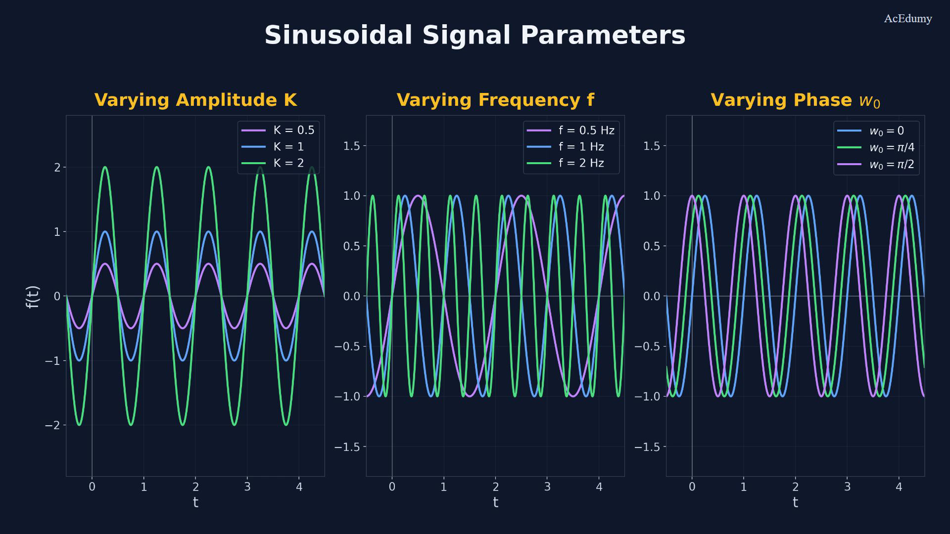
Original-video reference. In the sinusoid graph the purple arrow marks the time advance associated with phase. In the exponential comparison the far-left green segment is capped at 7.5 by the plotting code; the actual exponential continues growing as time tends to negative infinity. The damped graph is captured before the later erroneous peak markers appear; its formula is developed in the notebook lines.
Compare one parameter at a time.
Amplitude examples:
$\displaystyle K=0.5,1,2$
Increasing positive amplitude scales the waveform vertically.
Frequency examples in hertz:
$\displaystyle f=0.5,1,2$
Higher positive frequency gives more cycles and a shorter period.
Phase examples in radians:
$\displaystyle w_{0}=0,\frac{\pi }{4},\frac{\pi }{2}$
Changing phase preserves the amplitude and frequency.
Amplitude, frequency and phase specify the sinusoid; phase is equivalent modulo a full cycle.
Narration transcript
Let's compare how each parameter affects the waveform. In the first panel, we vary the amplitude K while keeping frequency and phase constant. A larger K stretches the wave vertically. In the second panel, we change the frequency. Higher frequency means more cycles packed into the same time interval, and a shorter period. In the third panel, we adjust the phase angle. The wave shifts horizontally, but its amplitude and frequency stay the same. These three parameters — amplitude, frequency, and phase — completely determine any sinusoidal signal.
4. Define a decaying exponential
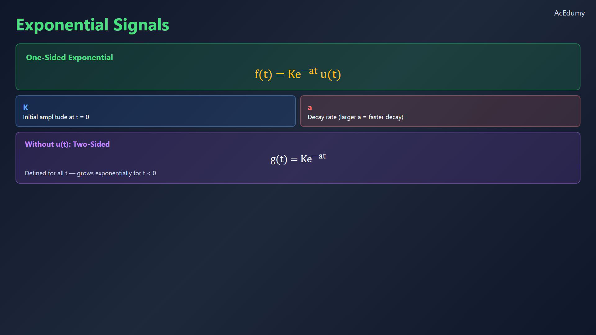
Original-video reference. In the sinusoid graph the purple arrow marks the time advance associated with phase. In the exponential comparison the far-left green segment is capped at 7.5 by the plotting code; the actual exponential continues growing as time tends to negative infinity. The damped graph is captured before the later erroneous peak markers appear; its formula is developed in the notebook lines.
Define a decaying exponential with positive decay rate.
One-sided exponential:
$\displaystyle f\left(t\right)=K e^{-a t} u\left(t\right)$
With the chosen unit-step convention:
$\displaystyle f\left(0\right)=K$
Larger positive decay rate means a shorter time constant:
$\displaystyle \tau =\frac{1}{a}$
For negative time:
$\displaystyle f\left(t\right)=0$
Without the unit step:
$\displaystyle g\left(t\right)=K e^{-a t}$
Narration transcript
The second signal type is the exponential signal. The one-sided form is f of t equals K e to the negative a t times u of t. Here K is the initial amplitude at t equals zero, and a is the decay rate. A larger value of a means faster decay. The unit step function u of t ensures the signal exists only for t greater than or equal to zero. Without the unit step, we get g of t equals K e to the negative a t, which is defined for all time — it grows exponentially for negative t values.
5. Compare one-sided and two-sided exponentials
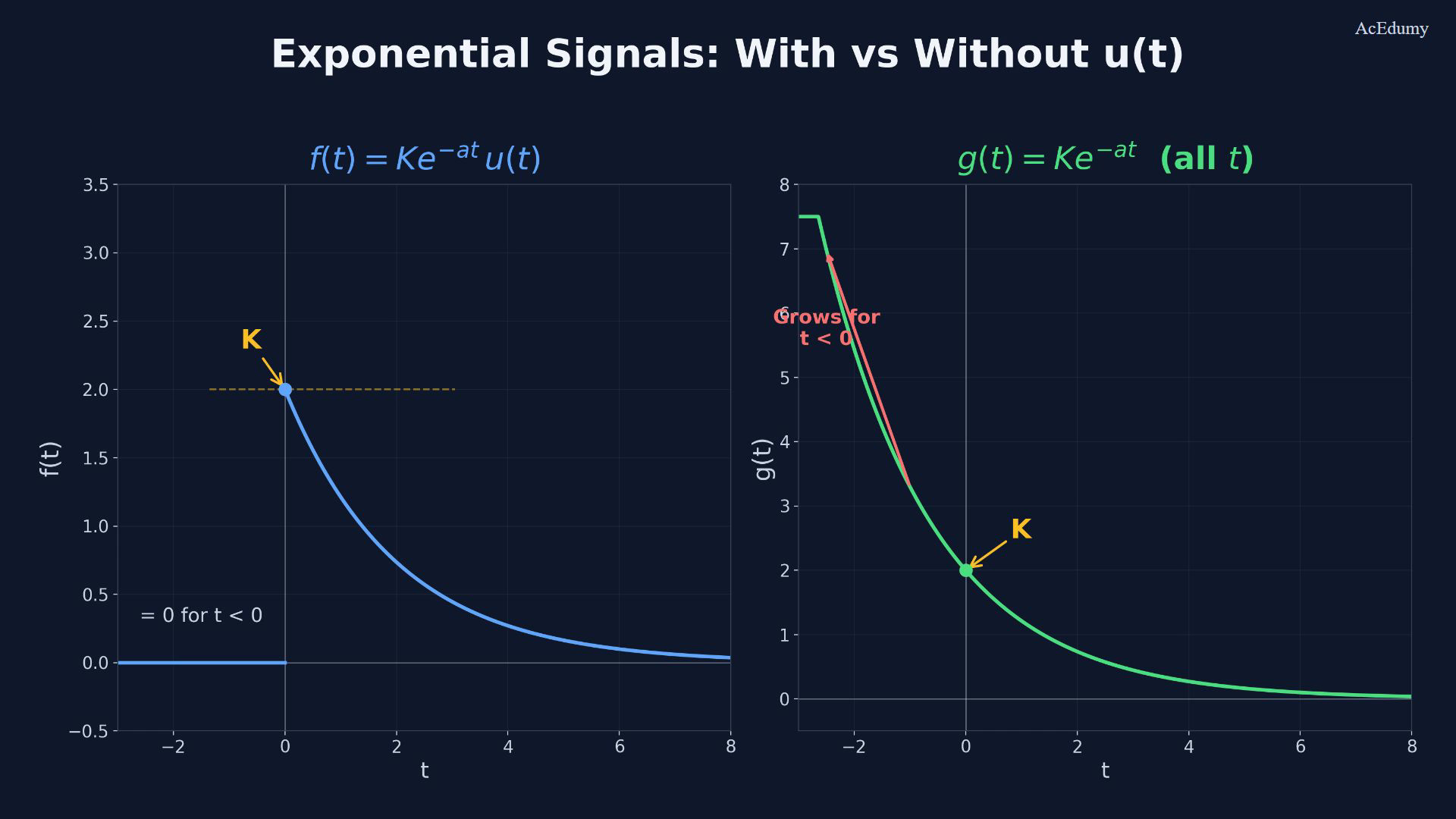
Original-video reference. In the sinusoid graph the purple arrow marks the time advance associated with phase. In the exponential comparison the far-left green segment is capped at 7.5 by the plotting code; the actual exponential continues growing as time tends to negative infinity. The damped graph is captured before the later erroneous peak markers appear; its formula is developed in the notebook lines.
Compare the two exponential equations and their time support.
Left graph:
$\displaystyle f\left(t\right)=K e^{-a t} u\left(t\right)$
Initial value under the chosen convention:
$\displaystyle f\left(0\right)=K$
For t<0:
$\displaystyle f\left(t\right)=0$
Right graph:
$\displaystyle g\left(t\right)=K e^{-a t}$
Toward increasingly negative times, for positive b:
$\displaystyle g\left(-b\right)=K e^{a b}$
The one-sided form models decay beginning at a finite starting time.
Narration transcript
Let's compare these two exponential forms side by side. On the left, f of t equals K e to the negative a t times u of t. The signal starts at K when t equals zero and decays smoothly toward zero. For negative time, the signal is exactly zero thanks to the unit step. On the right, g of t equals K e to the negative a t without the unit step. For positive t it looks identical, but for negative t it grows without bound. In practice, the one-sided exponential with u of t is far more common in physical systems.
6. Describe a damped sinusoid
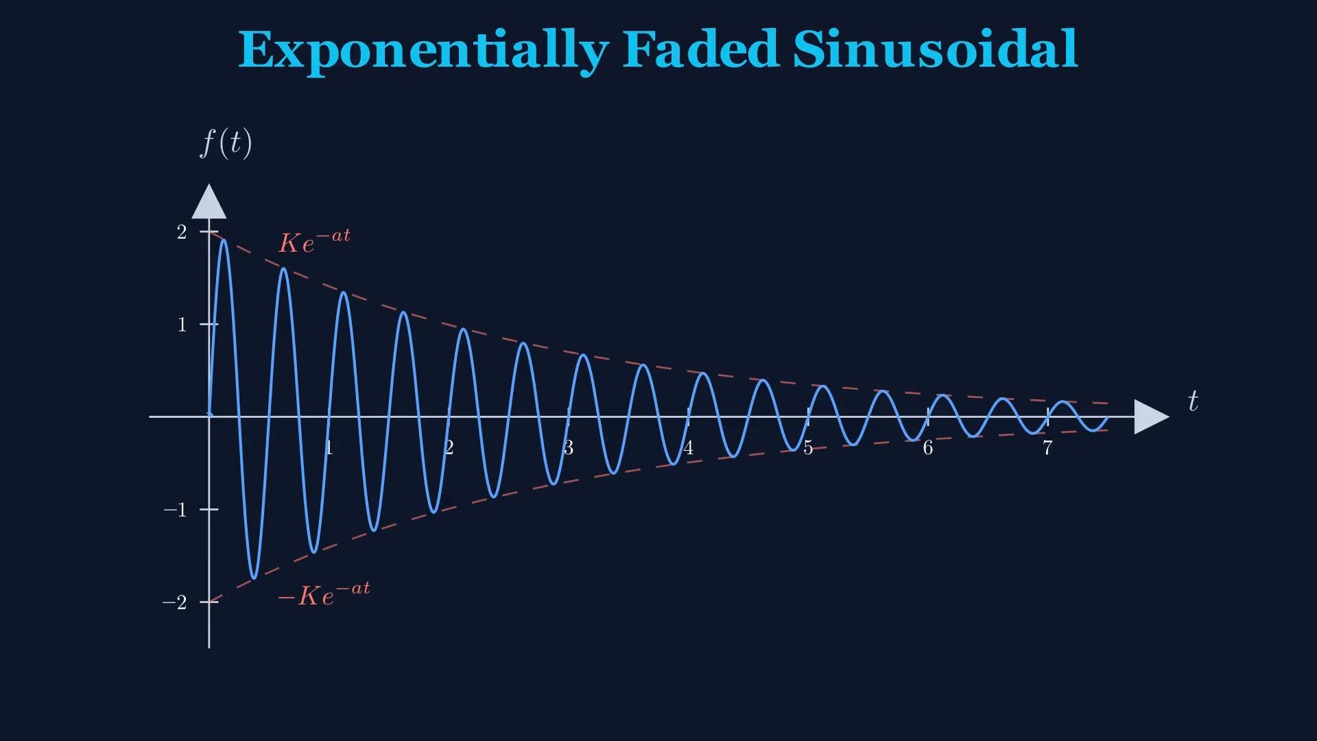
Original-video reference. In the sinusoid graph the purple arrow marks the time advance associated with phase. In the exponential comparison the far-left green segment is capped at 7.5 by the plotting code; the actual exponential continues growing as time tends to negative infinity. The damped graph is captured before the later erroneous peak markers appear; its formula is developed in the notebook lines.
Combine a sinusoidal oscillation with an exponential envelope.
Damped sinusoid:
$\displaystyle f\left(t\right)=K e^{-a t} \sin \left(\omega t+w_{0}\right) u\left(t\right)$
For nonnegative time, positive envelope:
$\displaystyle E\left(t\right)=K e^{-a t}$
Ratio of consecutive positive peak heights:
$\displaystyle \frac{P_{n+1}}{P_{n}}=e^{-a T}$
Examples include the free or transient response of an underdamped spring or RLC circuit.
Narration transcript
Our third signal type combines both concepts: the exponentially faded sinusoidal. It's defined as f of t equals K e to the negative a t times sine of omega t plus w zero, times u of t. The sinusoidal part creates the oscillation, while the exponential term K e to the negative a t acts as a decaying envelope. As time increases, each successive peak is smaller than the last. This signal appears naturally in many physical systems — an underdamped spring, an RLC circuit after a switch is closed, or any system that oscillates while losing energy.
7. Review the three signal types
Original-video reference. In the sinusoid graph the purple arrow marks the time advance associated with phase. In the exponential comparison the far-left green segment is capped at 7.5 by the plotting code; the actual exponential continues growing as time tends to negative infinity. The damped graph is captured before the later erroneous peak markers appear; its formula is developed in the notebook lines.
Review the three continuous-time signal types.
Sinusoid:
$\displaystyle f\left(t\right)=K \sin \left(\omega t+w_{0}\right)$
One-sided exponential:
$\displaystyle f\left(t\right)=K e^{-a t} u\left(t\right)$
Damped oscillation:
$\displaystyle f\left(t\right)=K e^{-a t} \sin \left(\omega t+w_{0}\right) u\left(t\right)$
Next: discrete-time signals and even-odd decomposition.
Narration transcript
Today we covered three continuous-time signal types. Sinusoidal signals are defined by amplitude K, frequency f or omega, and phase w zero. The exponential signal K e to the negative a t u of t models one-sided decay, while removing the unit step gives a two-sided exponential. The exponentially faded sinusoidal combines oscillation with decay, capturing the behavior of many real-world damped systems. In the next lesson, we'll review discrete-time signals and explore even-odd decomposition.