Signals and Systems · Convolution properties and the continuous-time integral

#15 Shifted impulses, signal decomposition and two-step convolution

Use convolution properties to combine shifted impulses, reconstruct a discrete sequence, and derive the ramp from two continuous-time unit steps.

Question

Original final-video graph or reference card for convolution properties. — Original-video reference. In the impulse-sum graph the six samples occupy integer indices negative two through three; the vertical axis marks index zero. The CT graph fixes output time at four: the shaded overlap is zero through four in the integration variable, and its area is four. The lower graph shows the ramp accumulated up to that time.

The star denotes convolution, while adjacent factors or a centered dot denote ordinary multiplication. For general signals, apply convolution identities where the defining sums or integrals exist; the finite DT examples and the CT step overlap here are well-defined. Linearity holds in either argument with the other fixed. The unshifted impulse is the identity; a shifted impulse translates the sequence by an integer index. In the DT impulse example y names the second input; in the CT section y names the output. The six-sample decomposition starts at index negative two and is zero outside indices negative two through three. Keep n and the summation index k separate; keep output time t fixed when integrating over tau. Choose u(0)=1 as in the narration, although changing a single endpoint value does not alter the CT integral. For the two-step CT example, negative output time gives no overlap and zero output. The integral from zero to t applies only for nonnegative output time, including zero where its interval has zero length. The CT reference fixes output time at four, while the conditional integral describes every nonnegative output time.

Written solution and narration transcript(shows the full solution)

Below are all the lines written in the notebook together with the full narration transcript.

1. DT convolution properties
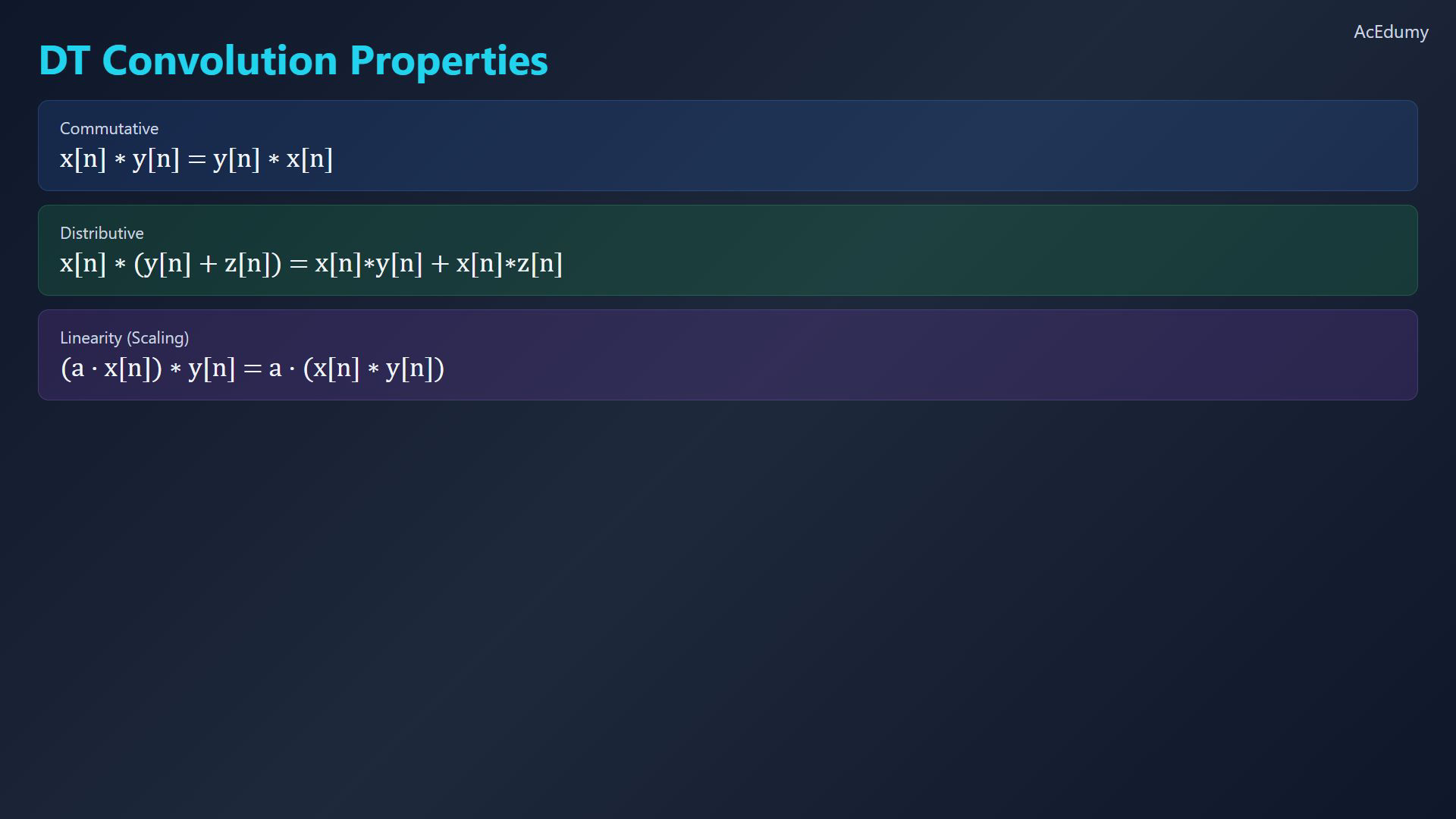
Original-video reference. In the impulse-sum graph the six samples occupy integer indices negative two through three; the vertical axis marks index zero. The CT graph fixes output time at four: the shaded overlap is zero through four in the integration variable, and its area is four. The lower graph shows the ramp accumulated up to that time.
Three useful properties of discrete-time convolution.
Commutativity:
$\displaystyle x\left[n\right]∗y\left[n\right]=y\left[n\right]∗x\left[n\right]$
The order of the two input sequences does not change the result.
Distributivity:
$\displaystyle x\left[n\right]∗\left(y\left[n\right]+z\left[n\right]\right)=x\left[n\right]∗y\left[n\right]+x\left[n\right]∗z\left[n\right]$
Scaling with the other argument fixed:
$\displaystyle \left(a x\left[n\right]\right)∗y\left[n\right]=a\left(x\left[n\right]∗y\left[n\right]\right)$
Distributivity and scaling give linearity in either argument separately.
Narration transcript
Let's explore the key properties of discrete-time convolution. First, commutativity: x of n convolved with y of n equals y of n convolved with x of n. The order doesn't matter. Second, distributivity: x of n convolved with the sum y of n plus z of n, can be split into separate convolutions and then added together. Third, linearity: scaling a signal before convolution is the same as scaling the result after convolution. These three properties together make convolution a powerful and flexible operation.
2. Shifted impulse
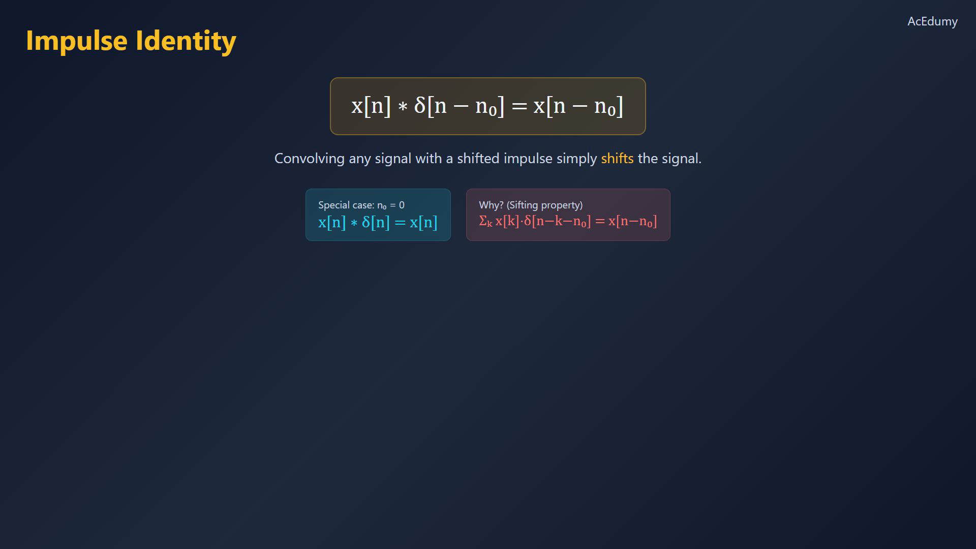
Original-video reference. In the impulse-sum graph the six samples occupy integer indices negative two through three; the vertical axis marks index zero. The CT graph fixes output time at four: the shaded overlap is zero through four in the integration variable, and its area is four. The lower graph shows the ramp accumulated up to that time.
Convolution with a discrete impulse gives a simple shift.
For an integer shift:
$\displaystyle x\left[n\right]∗\delta \left[n-n_{0}\right]=x\left[n-n_{0}\right]$
Sifting selects the input sample at the shifted index.
The unshifted impulse is the identity:
$\displaystyle x\left[n\right]∗\delta \left[n\right]=x\left[n\right]$
Narration transcript
Perhaps the most important property involves the impulse function. When you convolve any signal x of n with a shifted impulse delta of n minus n zero, the result is simply x of n minus n zero, the original signal shifted by n zero. This follows directly from the sifting property of the impulse. The impulse acts as the identity element for convolution, just like multiplying by one in arithmetic.
3. Two shifted impulses
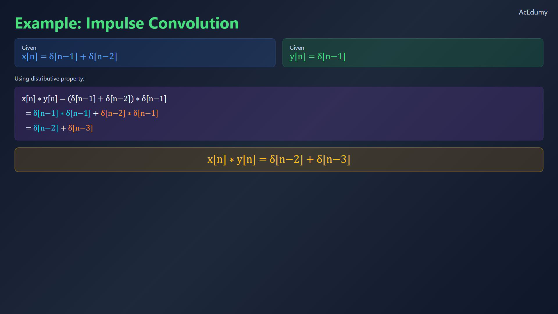
Original-video reference. In the impulse-sum graph the six samples occupy integer indices negative two through three; the vertical axis marks index zero. The CT graph fixes output time at four: the shaded overlap is zero through four in the integration variable, and its area is four. The lower graph shows the ramp accumulated up to that time.
Apply the impulse and distributive properties.
Given two input sequences:
$\displaystyle x\left[n\right]=\delta \left[n-1\right]+\delta \left[n-2\right], y\left[n\right]=\delta \left[n-1\right]$
Split the sum into two separate impulse convolutions.
First term:
$\displaystyle \delta \left[n-1\right]∗\delta \left[n-1\right]=\delta \left[n-2\right]$
Second term:
$\displaystyle \delta \left[n-2\right]∗\delta \left[n-1\right]=\delta \left[n-3\right]$
Add the two terms:
$\displaystyle x\left[n\right]∗y\left[n\right]=\delta \left[n-2\right]+\delta \left[n-3\right]$
Narration transcript
Let's apply these properties. Given x of n equals delta of n minus one plus delta of n minus two, and y of n equals delta of n minus one. Using the distributive property, we split the convolution into two parts. Delta of n minus one convolved with delta of n minus one: by the impulse identity, this gives delta of n minus two. Delta of n minus two convolved with delta of n minus one: this gives delta of n minus three. So the final result is delta of n minus two plus delta of n minus three.
4. Signal decomposition
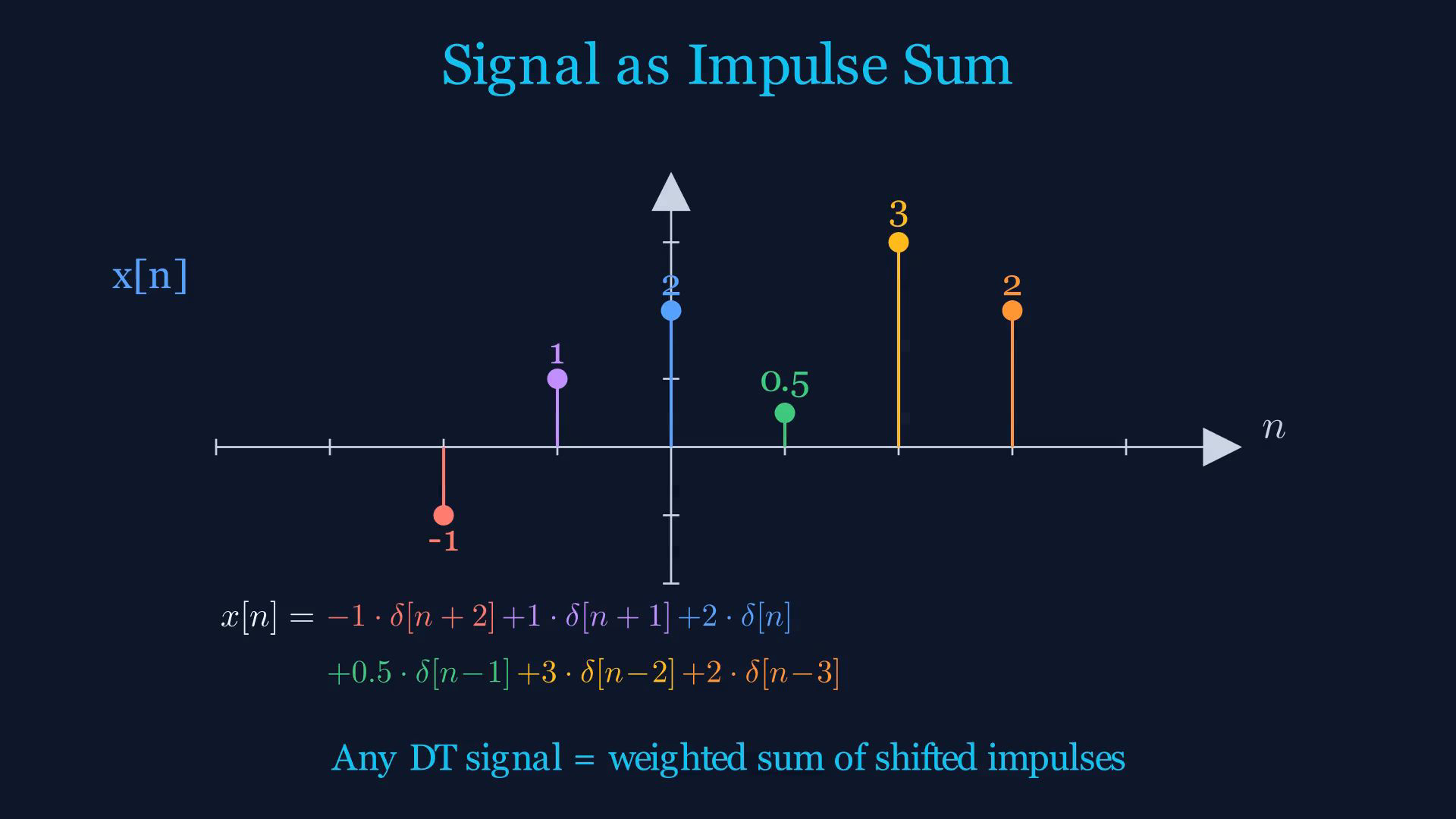
Original-video reference. In the impulse-sum graph the six samples occupy integer indices negative two through three; the vertical axis marks index zero. The CT graph fixes output time at four: the shaded overlap is zero through four in the integration variable, and its area is four. The lower graph shows the ramp accumulated up to that time.
A signal can be reconstructed sample by sample.
Impulse expansion:
$\displaystyle x\left[n\right]=\sum _{k=-\infty }^{\infty } x\left[k\right]\delta \left[n-k\right]$
Values indexed negative two through three:
$\displaystyle x=\left[-1,1,2,0.5,3,2\right]$
Weighted impulse expansion:
$\displaystyle x\left[n\right]=-\delta \left[n+2\right]+\delta \left[n+1\right]+2\delta \left[n\right]+0.5\delta \left[n-1\right]+3\delta \left[n-2\right]+2\delta \left[n-3\right]$
This decomposition explains why convolution is a sum of shifted responses.
Narration transcript
Here's a fundamental insight. Any discrete-time signal can be written as a weighted sum of shifted impulse functions. For example, consider x of n with values negative one, one, two, zero point five, three, two, starting at n equals negative two. We write this as: negative one times delta of n plus two, plus one times delta of n plus one, plus two times delta of n, plus zero point five times delta of n minus one, plus three times delta of n minus two, plus two times delta of n minus three. This decomposition is the foundation of the convolution sum.
5. CT convolution integral
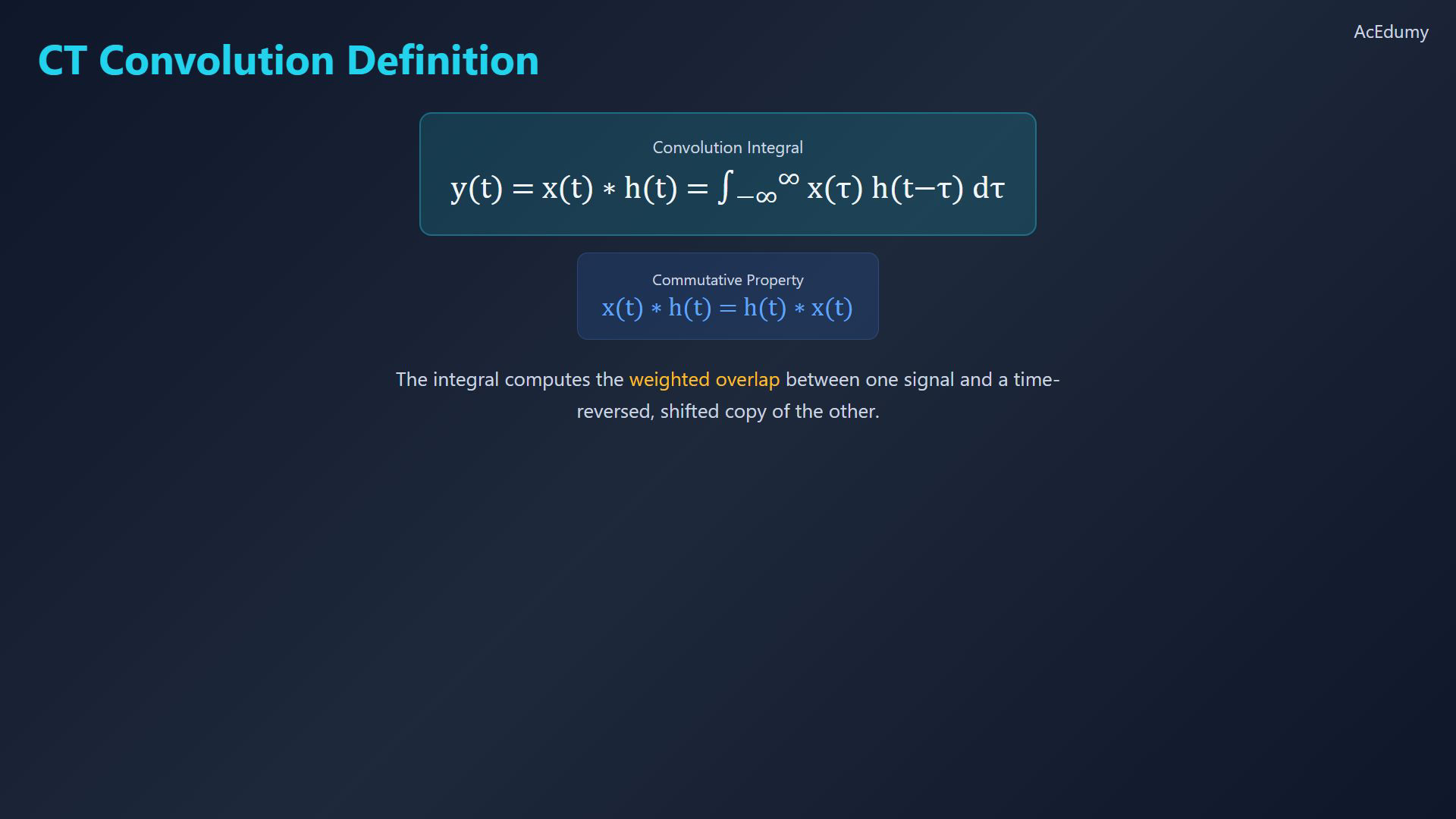
Original-video reference. In the impulse-sum graph the six samples occupy integer indices negative two through three; the vertical axis marks index zero. The CT graph fixes output time at four: the shaded overlap is zero through four in the integration variable, and its area is four. The lower graph shows the ramp accumulated up to that time.
Replace the discrete sum with a continuous-time integral.
CT convolution:
$\displaystyle y\left(t\right)=\int _{-\infty }^{\infty } x\left(\tau \right)h\left(t-\tau \right)\mathrm{d}\tau$
Commutativity:
$\displaystyle x\left(t\right)∗h\left(t\right)=h\left(t\right)∗x\left(t\right)$
At fixed output time, integrate the weighted overlap with a reversed and shifted signal.
Narration transcript
Now let's move to continuous-time convolution. For C T signals x of t and h of t, the convolution is defined as y of t equals the integral from negative infinity to positive infinity of x of tau times h of t minus tau, d tau. Just like in discrete time, C T convolution is commutative: x of t convolved with h of t equals h of t convolved with x of t. This integral computes the weighted overlap between one signal and a time-reversed, shifted copy of the other.
6. Two unit steps
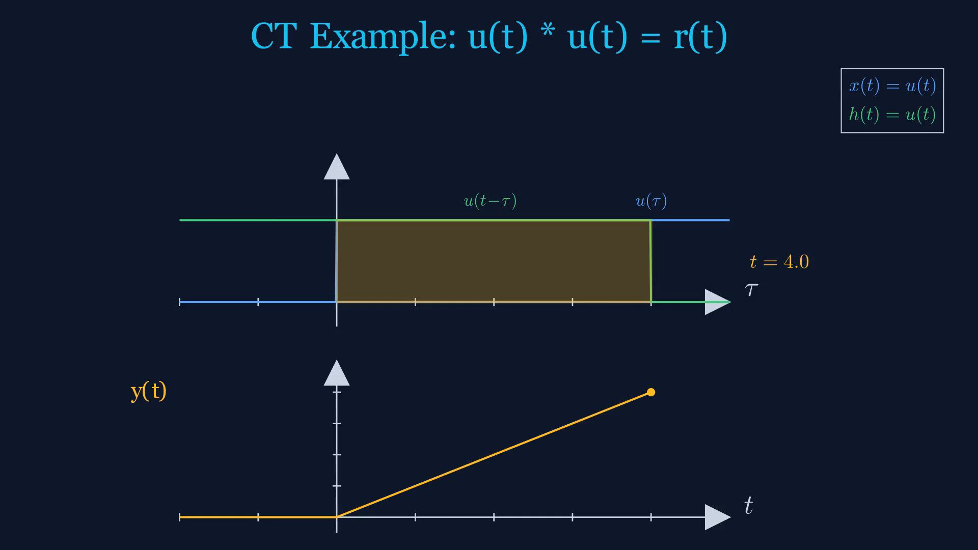
Original-video reference. In the impulse-sum graph the six samples occupy integer indices negative two through three; the vertical axis marks index zero. The CT graph fixes output time at four: the shaded overlap is zero through four in the integration variable, and its area is four. The lower graph shows the ramp accumulated up to that time.
Convolve two unit steps:
$\displaystyle y\left(t\right)=u\left(t\right)∗u\left(t\right)$
Start from the full integral:
$\displaystyle y\left(t\right)=\int _{-\infty }^{\infty }u\left(\tau \right)u\left(t-\tau \right)\mathrm{d}\tau$
The first step is one for nonnegative integration variable and zero otherwise.
The reversed shifted step is one when the integration variable is no greater than output time.
Both factors are one only on the interval from zero to nonnegative output time; negative output time gives no overlap.
For nonnegative output time:
$\displaystyle y\left(t\right)=\int _{0}^{t} 1d\tau =t$
For all real output times:
$\displaystyle y\left(t\right)=t u\left(t\right)=r\left(t\right)$
Narration transcript
Let's compute our first C T convolution: u of t convolved with u of t. Setting up the integral, we need u of tau, times u of t minus tau. u of tau equals one for tau greater than or equal to zero, and zero otherwise. u of t minus tau equals one when tau is less than or equal to t, and zero otherwise. Their product is one only when zero is less than or equal to tau, and tau is less than or equal to t. The integral becomes the integral from zero to t of one d tau, which equals t, for t greater than or equal to zero. Therefore, u of t convolved with u of t equals t times u of t, which is the ramp function r of t.
7. Summary
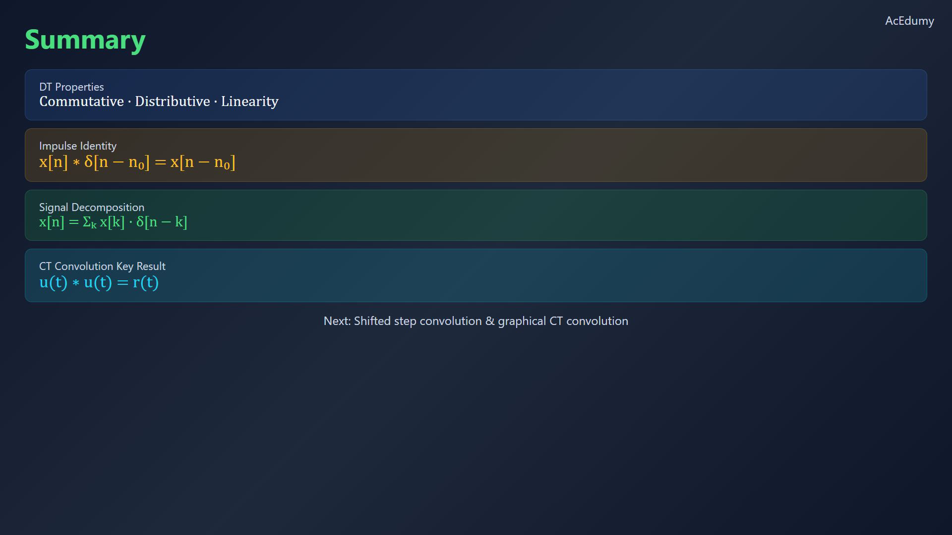
Original-video reference. In the impulse-sum graph the six samples occupy integer indices negative two through three; the vertical axis marks index zero. The CT graph fixes output time at four: the shaded overlap is zero through four in the integration variable, and its area is four. The lower graph shows the ramp accumulated up to that time.
Convolution is commutative, distributive, and linear in each argument separately.
Integer impulse shift:
$\displaystyle x\left[n\right]∗\delta \left[n-n_{0}\right]=x\left[n-n_{0}\right]$
A DT signal is the weighted sum of its shifted impulses.
Two CT unit steps give the ramp:
$\displaystyle u\left(t\right)∗u\left(t\right)=r\left(t\right)$
Next: shifted step convolutions and graphical examples.
Narration transcript
Today we learned the three key properties of D T convolution: commutativity, distributivity, and linearity. The impulse identity, x of n convolved with delta of n minus n zero equals x of n minus n zero, is especially powerful. Any signal can be decomposed into a weighted sum of shifted impulses. We also introduced C T convolution as an integral and showed that the convolution of two unit steps equals the ramp function. In the next lesson, we'll extend C T convolution to shifted steps and work through graphical convolution examples.