Signals and Systems · Continuous and discrete impulse functions
#08 Unit area, sifting, multiplication and nonzero-slope scaling
Distinguish continuous impulse weight from a discrete unit sample; evaluate polynomial sifting and multiplication examples, then track both location and absolute-slope weight.
Question
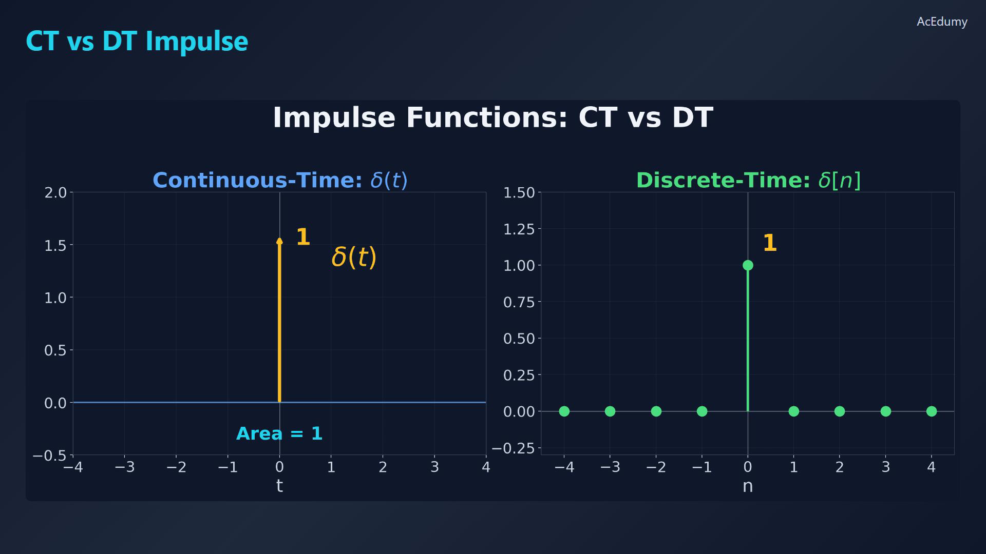
Treat the CT Dirac impulse as a unit point mass/distribution, not an ordinary function with an infinite point value. The narrowing rectangular approximation has positive width Δ, height1/Δ and area1; its convergence is distributional. The source's infinite-at-zero wording is only a heuristic limiting picture, clarified visibly without altering narration. Its smoothed unit step is a finite transition from zero to one, not the unbounded unit ramp. CT arrows label weight, not literal height. The DT Kronecker sequence has δ[0]=1 andδ[n]=0 at other integers; discrete sifting uses a sum. For CT sifting and multiplication require a factor regular in a neighborhood of the impulse, as in all polynomial examples and the step away from its jump. Do not apply an unqualified any-function rule at a singularity or discontinuity. The integral of δ(t−1)(2t²+1) is3. Multiplication δ(t−1)(2t³−1) isδ(t−1). δ(t−1)u(t−2) is zero because the step is locally identically zero near t=1; its convention at t=2 is irrelevant. For real a≠0,δ(a t)=δ(t)/|a|; negative a still has a positive weight. The source's unchanged location statement is restricted to the unshifted impulse at the origin, not shifted arguments. δ(2t−1)=δ(t−1/2)/2 andδ(3t−3)=δ(t−1)/3. In general the root of a t−b is b/a and the weight is1/|a|. Exclude a=0; do not transfer the CT Jacobian to DT Kronecker samples: for nonzero integer M,δ[M n]=δ[n],without1/|M|. Source narration remains literal. Existing final only; no source generator or embedded credential was executed. Seven final-derived MP3s and final correlations are same-source extraction integrity, not independent original TTS provenance. All47 source/large cue lines and all7 cached-small text,segments and word times read; large confidence .7744–1 and small .896–1 under unchanged .62 gate. Large multiplication omits some arguments, which small recovers; small stem-plot phonetics and summary Delta repetition are model output differences, not proof of incorrect spoken source. All7 actual final frames inspected; the clipped limit integral is replaced by the clean original CT/DT frame at114.600s. Seven roles use six unique original frames, with unchanged pixels. No whole-final ASR or complete human listening/pedagogy/motion/publication approval is claimed. Unpublished technical draft only. No new TTS, paid generation, model downloads, video render/upload/publication, access/deploy/Play/ports/security/egress changes or legacy single-JSON import.
Written solution and narration transcript(shows the full solution)
Below are all the lines written in the notebook together with the full narration transcript.
1. Keep unit area while a rectangular pulse narrows
Original-video reference. The limit section uses the clean CT/DT unit-area comparison because its original limit panel clips the integral. The CT arrow label denotes impulse weight, not ordinary function height. Other panels are unchanged original frames; continuous-time scaling assumes a nonzero real slope and is not the discrete Kronecker scaling rule. The continuous-time unit impulse is an idealized unit point mass.Start with a smoothed unit step, not an unbounded unit ramp.Let its transition from zero to one have positive width Δ.The derivative pulse has reciprocal height:Its area is independent of positive width:Take the limit as the positive width decreases to zero, in the distributional sense.Every approximating pulse has unit area:The infinite-peak description is a limiting picture; δ is a distribution, not an ordinary function with an infinite point value.The arrow label one denotes impulse weight, not a finite or infinite plotted height.Narration transcript
The impulse function delta of t is perhaps the most unusual signal you will encounter. To define it, we start with a gentler version. Consider u sub delta of t, a ramp that rises from zero to one over an interval of width delta. Its derivative, delta sub delta of t, is a rectangular pulse of height one over delta and width delta. The crucial property is that its area equals one, regardless of how small delta is. Now take the limit as delta approaches zero. The pulse gets narrower and taller, but its area remains exactly one. In the limit, we get the unit impulse delta of t: zero everywhere except at t equals zero, where it is infinite, yet its total area is still one. We draw it as an upward arrow at the origin with a label of one.
2. Define the ordinary discrete-time unit sample
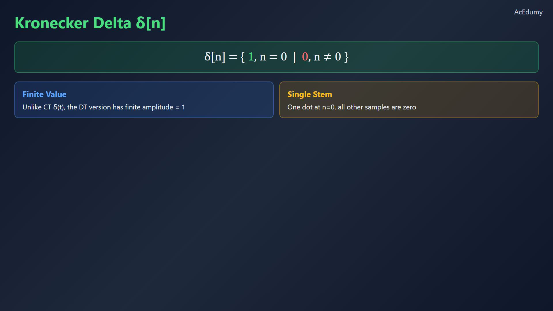
Original-video reference. The limit section uses the clean CT/DT unit-area comparison because its original limit panel clips the integral. The CT arrow label denotes impulse weight, not ordinary function height. Other panels are unchanged original frames; continuous-time scaling assumes a nonzero real slope and is not the discrete Kronecker scaling rule. The discrete-time unit sample is an ordinary sequence.At zero it is one, and at every other integer it is zero:Its amplitude at zero is finite.Draw a stem of height one at the zero index and zero elsewhere.Its discrete sifting rule uses a sum, not a continuous-time integral.Narration transcript
The discrete-time counterpart is much simpler. The Kronecker delta, delta of n, equals one when n is zero and zero for all other integers. Unlike the continuous-time impulse, it has a finite value. Its stem plot is a single dot at height one above n equals zero, with all other values at zero. Despite its simplicity, it plays the same fundamental role in discrete-time signal processing that delta of t plays in continuous time.
3. Distinguish impulse weight from sample amplitude
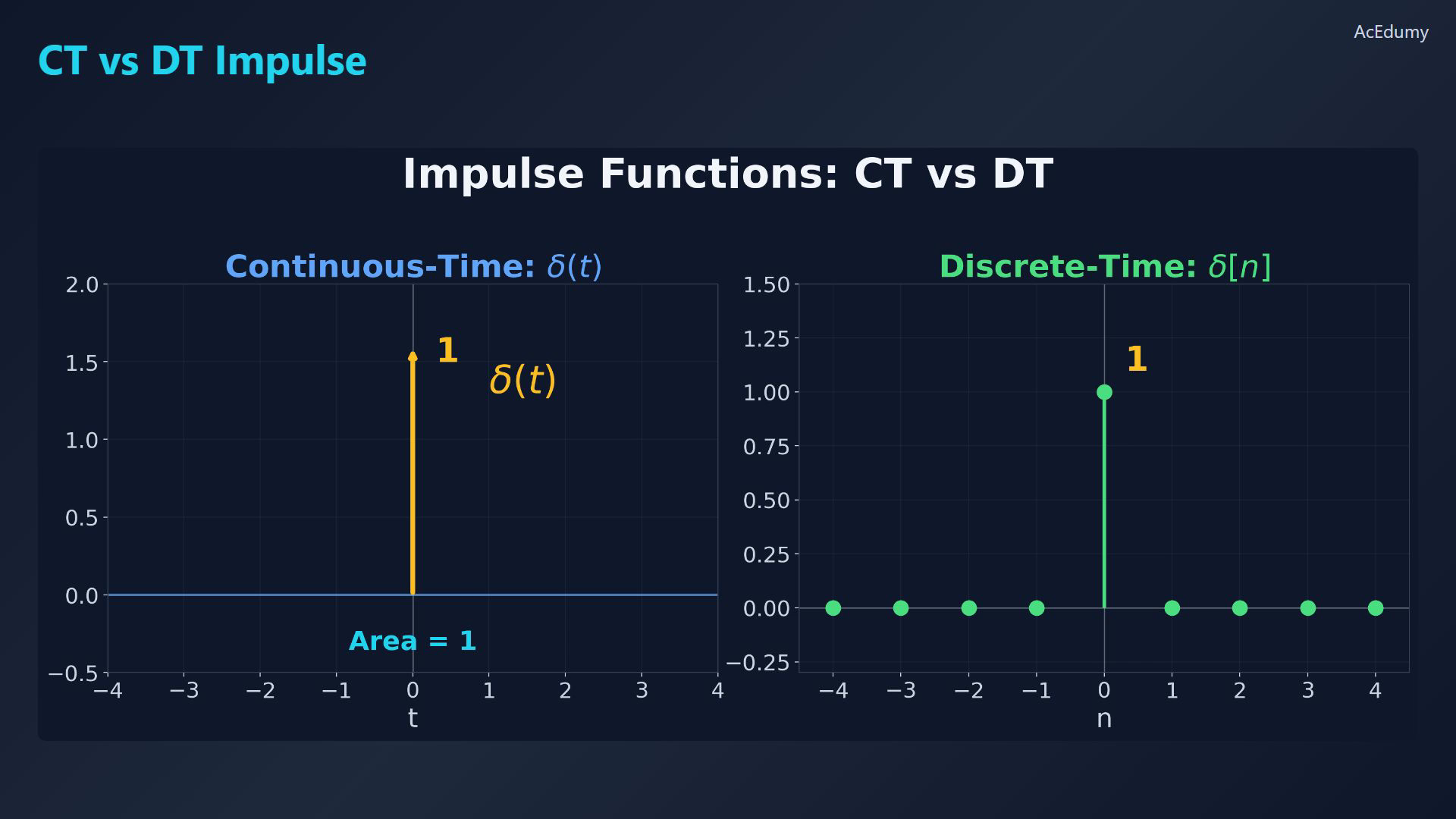
Original-video reference. The limit section uses the clean CT/DT unit-area comparison because its original limit panel clips the integral. The CT arrow label denotes impulse weight, not ordinary function height. Other panels are unchanged original frames; continuous-time scaling assumes a nonzero real slope and is not the discrete Kronecker scaling rule. The CT arrow label is unit weight; the DT stem height is an actual sample value of one.A physical CT pulse can approximate an ideal impulse; the DT unit sample is already a finite-valued sequence.Both select values, but the CT rule uses an integral and the DT rule uses a sum.Narration transcript
Comparing the two impulse functions side by side: the CT impulse delta of t is represented by an arrow at the origin with unit area, while the DT impulse delta of n is a simple stem at n equals zero with value one. The CT version is a mathematical idealization that cannot be physically realized, while the DT version is a perfectly ordinary signal with finite amplitude. Both share the crucial sifting property that we will explore next.
4. Evaluate a polynomial at the impulse location
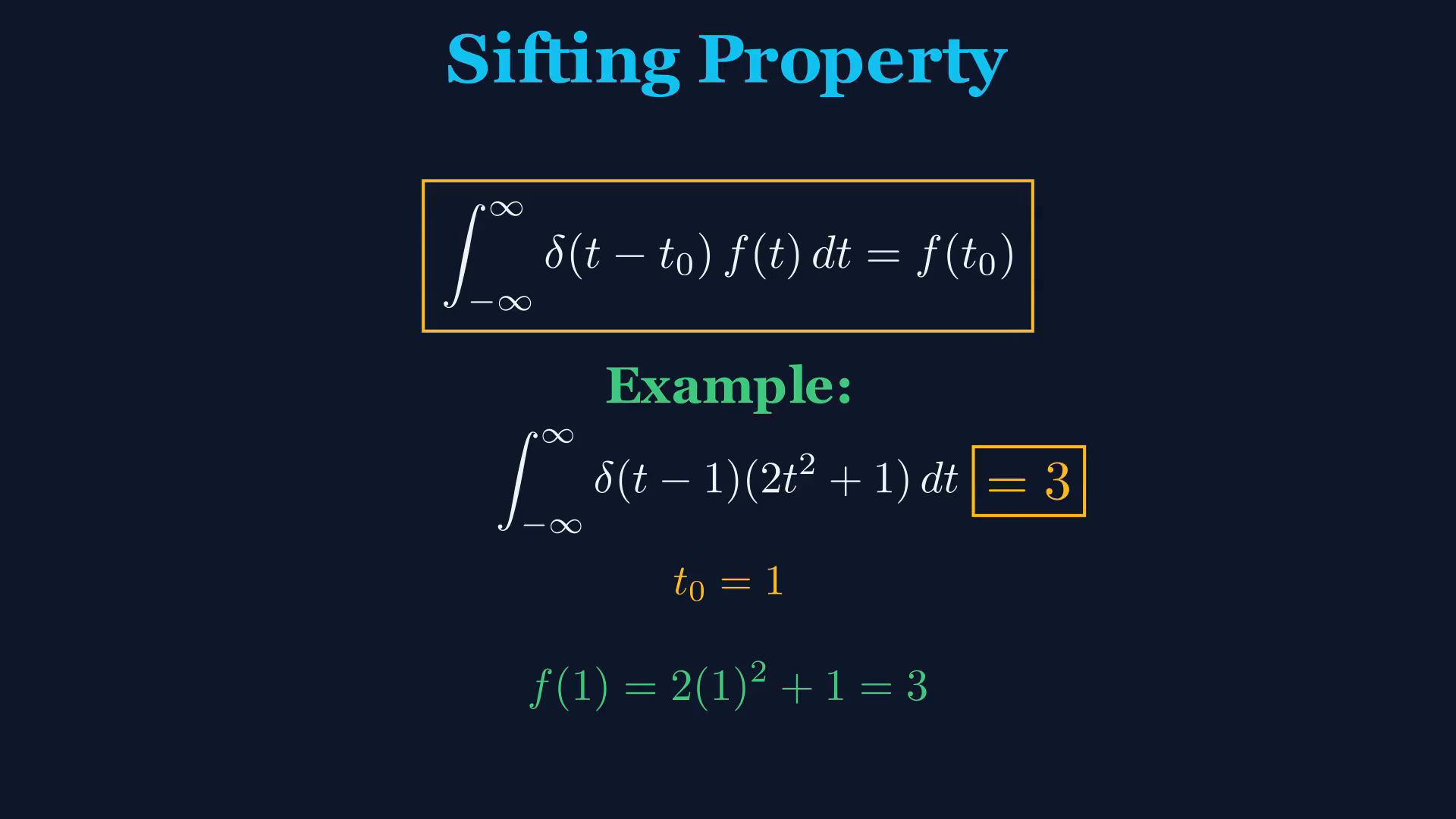
Original-video reference. The limit section uses the clean CT/DT unit-area comparison because its original limit panel clips the integral. The CT arrow label denotes impulse weight, not ordinary function height. Other panels are unchanged original frames; continuous-time scaling assumes a nonzero real slope and is not the discrete Kronecker scaling rule. Sifting extracts the value at the impulse location.For a factor regular near the impulse, use:The factor must be regular at that location; an arbitrary discontinuity or singularity needs additional care.Use a polynomial factor in this example.Evaluate the integral:Substitute the impulse location into the polynomial:Therefore the integral is:Narration transcript
The sifting property is the most important property of the impulse function. It states that the integral from negative infinity to infinity of delta of t minus t zero times f of t d t equals f of t zero. In words: multiplying any function by a shifted impulse and integrating extracts the function's value at the impulse location. Let us work through an example. Find the integral of delta of t minus one times the quantity two t squared plus one, d t. By the sifting property, we evaluate f of t at t equals one: f of one equals two times one squared plus one, which equals three. The entire integral equals three.
5. Freeze a locally regular factor at the impulse
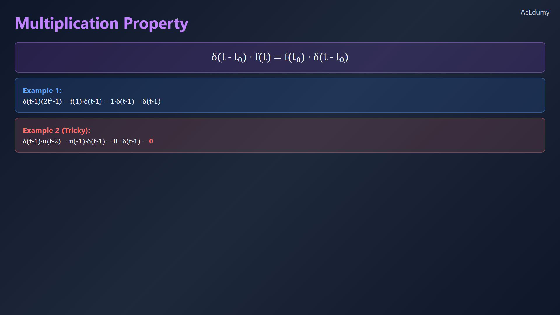
Original-video reference. The limit section uses the clean CT/DT unit-area comparison because its original limit panel clips the integral. The CT arrow label denotes impulse weight, not ordinary function height. Other panels are unchanged original frames; continuous-time scaling assumes a nonzero real slope and is not the discrete Kronecker scaling rule. Multiplication keeps the impulse and evaluates its regular factor.For a factor regular near the impulse:Only the factor value at the impulse location determines its resulting weight.Example with a polynomial factor:Evaluate at one:The unit-weight impulse remains:Now multiply by a step whose jump is elsewhere:The step is zero near the impulse location:Thus the product is the zero distribution:Narration transcript
A closely related property is the multiplication rule. When we multiply delta of t minus t zero by a function f of t, the result is f of t zero times delta of t minus t zero. The impulse freezes the function at its location. For example, delta of t minus one times two t cubed minus one. Since the impulse is at t equals one, we evaluate f of one equals two times one cubed minus one, which equals one. So the product simplifies to delta of t minus one. Here is a tricky example: delta of t minus one times u of t minus two. The impulse is at t equals one, so u of one minus two equals u of negative one, which is zero. The entire product is zero.
6. Scale strength by the absolute nonzero slope
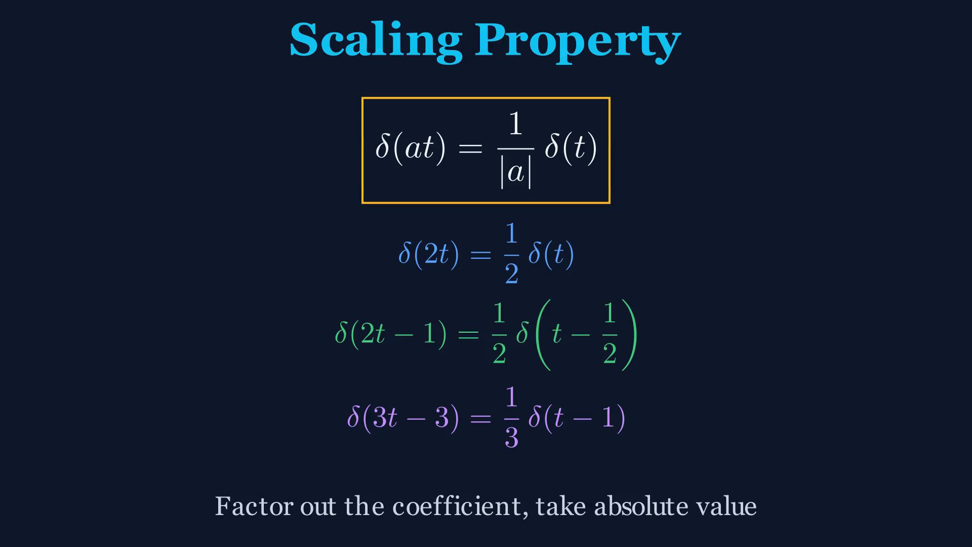
Original-video reference. The limit section uses the clean CT/DT unit-area comparison because its original limit panel clips the integral. The CT arrow label denotes impulse weight, not ordinary function height. Other panels are unchanged original frames; continuous-time scaling assumes a nonzero real slope and is not the discrete Kronecker scaling rule. For nonzero real slope, the continuous-time rule is:Only for the unshifted impulse at the origin does scaling leave its location unchanged.Positive slope two halves the weight:Negative slope also uses the absolute value:A shifted argument changes the location as well:Location and weight are both one half:The zero of the argument is one and the weight is one third:Narration transcript
The scaling property states that delta of a t equals one over the absolute value of a, times delta of t. Time-scaling an impulse only changes its strength, not its location. Delta of two t equals one half times delta of t. Delta of negative two t also equals one half delta of t, because we take the absolute value. For a shifted version: delta of two t minus one equals one half times delta of t minus one half. The impulse moves to t equals one half with strength one half. Similarly, delta of three t minus three equals one third times delta of t minus one.
7. Review the continuous and discrete impulse rules

Original-video reference. The limit section uses the clean CT/DT unit-area comparison because its original limit panel clips the integral. The CT arrow label denotes impulse weight, not ordinary function height. Other panels are unchanged original frames; continuous-time scaling assumes a nonzero real slope and is not the discrete Kronecker scaling rule. Review the impulse rules with their continuous or discrete domains.The continuous-time impulse is the distributional limit of narrowing unit-area pulses.The discrete unit sample is zero at other integers:Sifting evaluates a locally regular factor at the impulse location.Multiplication preserves the impulse and freezes its locally regular factor.For nonzero real slope in continuous time:Next, connect the elementary signals through derivatives and integrals.Narration transcript
Let us summarize. Delta of t is defined as the limit of narrowing pulses with unit area. Delta of n is simply one at n equals zero. The sifting property extracts function values: the integral of delta times f equals f at the impulse location. The multiplication property freezes functions at the impulse point. And the scaling property adjusts impulse strength: delta of a t equals one over absolute a times delta of t. Next, we will connect all three elementary signals through derivatives and integrals.
Source video: Signals & Systems #08 | Impulse Function delta(t) - Sifting, Multiplication & Scaling (5:06)