Signals and Systems · LTI differential and difference equations

#19 Homogeneous and particular solutions; recursive computation

Solve a second-order differential equation using homogeneous and particular terms, then compute three samples of a first-order difference equation.

Question

Original final-video reference for solving a differential or difference equation. — Original-video reference. The CT example shows the complete solution for a smooth exponential input. For the DT computation step, the reference is the general recursion card; the timed written lines give the three computed values. Read the simple-root and nonresonance assumptions in the problem statement.

Use finite-order linear constant-coefficient equations with nonzero leading output coefficient. The general CT model covers systems described by such equations, rather than every possible LTI operator. Work on an interval where the input is sufficiently differentiable. The CT example uses the smooth exponential exp(-t), with no implicit unit-step multiplier or switching impulse. Its constants are determined by applying the initial conditions to the full solution and its derivative. The input-output LTI description refers to the zero-state system; adding a fixed nonzero initial-condition response does not itself define a linear input-output map. For the displayed sum of homogeneous exponentials, assume distinct characteristic roots as in the worked example. Repeated roots require additional powers of time. The trial table gives nonresonant forms: zero must not be a root for its polynomial rows, and neither plus nor minus j omega may be a root for its sinusoidal row. The exponential row explicitly requires negative a not to be a root. The source card exception that multiplies by time is the simple-root case; a root of multiplicity m requires multiplication by time to the power m. The damped-sinusoid row uses cosine and sine of omega times time. Root signs describe natural-mode decay or growth; purely imaginary roots give oscillation, and complex growth refers to magnitude. For DT recursion, a sub zero is a nonzero coefficient, not the number zero; current-input terms start at index zero and past-output terms at index one. The source FIR card uses normalized coefficients with a sub zero equal to one. Use finite filter coefficients; feedback alone does not exclude pole-zero cancellation to a finite impulse response. In the DT example, the unit step equals one at zero and for positive integer indices, and zero at negative indices; the initial output at negative one is zero. The final DT table clips its left index column, so the defter uses the complete recursion card as its reference and explicitly labels every computed output in the timed text.

Written solution and narration transcript(shows the full solution)

Below are all the lines written in the notebook together with the full narration transcript.

1. CT differential equations
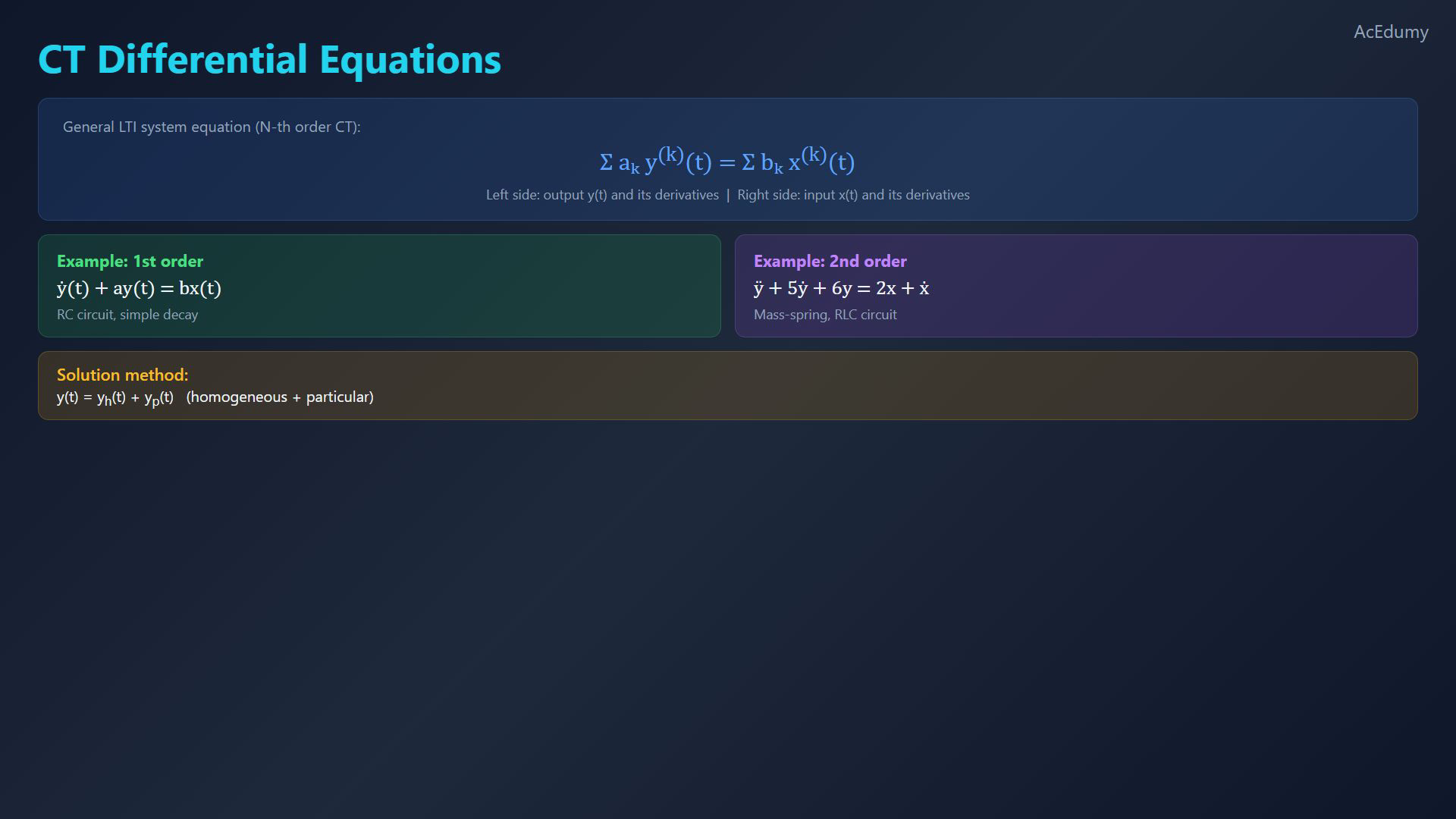
Original-video reference. The CT example shows the complete solution for a smooth exponential input. For the DT computation step, the reference is the general recursion card; the timed written lines give the three computed values. Read the simple-root and nonresonance assumptions in the problem statement.
Describe finite-order LTI systems with differential and difference equations.
CT equation with constant coefficients:
$\displaystyle \sum _{k=0}^{N}a_{k} y^{(k)}\left(t\right)=\sum _{k=0}^{M}b_{k} x^{(k)}\left(t\right)$
The left side contains output derivatives; the right side contains input derivatives.
Find the output from the input and the initial conditions.
Narration transcript
In this lesson we explore how LTI systems are described by differential and difference equations. For a continuous-time LTI system, the input output relationship takes the general form: the sum of a sub k times the k-th derivative of y, equals the sum of b sub k times the k-th derivative of x. The left side involves the output y of t and its derivatives, while the right side involves the input x of t and its derivatives. Our goal is to find y given x and the initial conditions.
2. Homogeneous solution
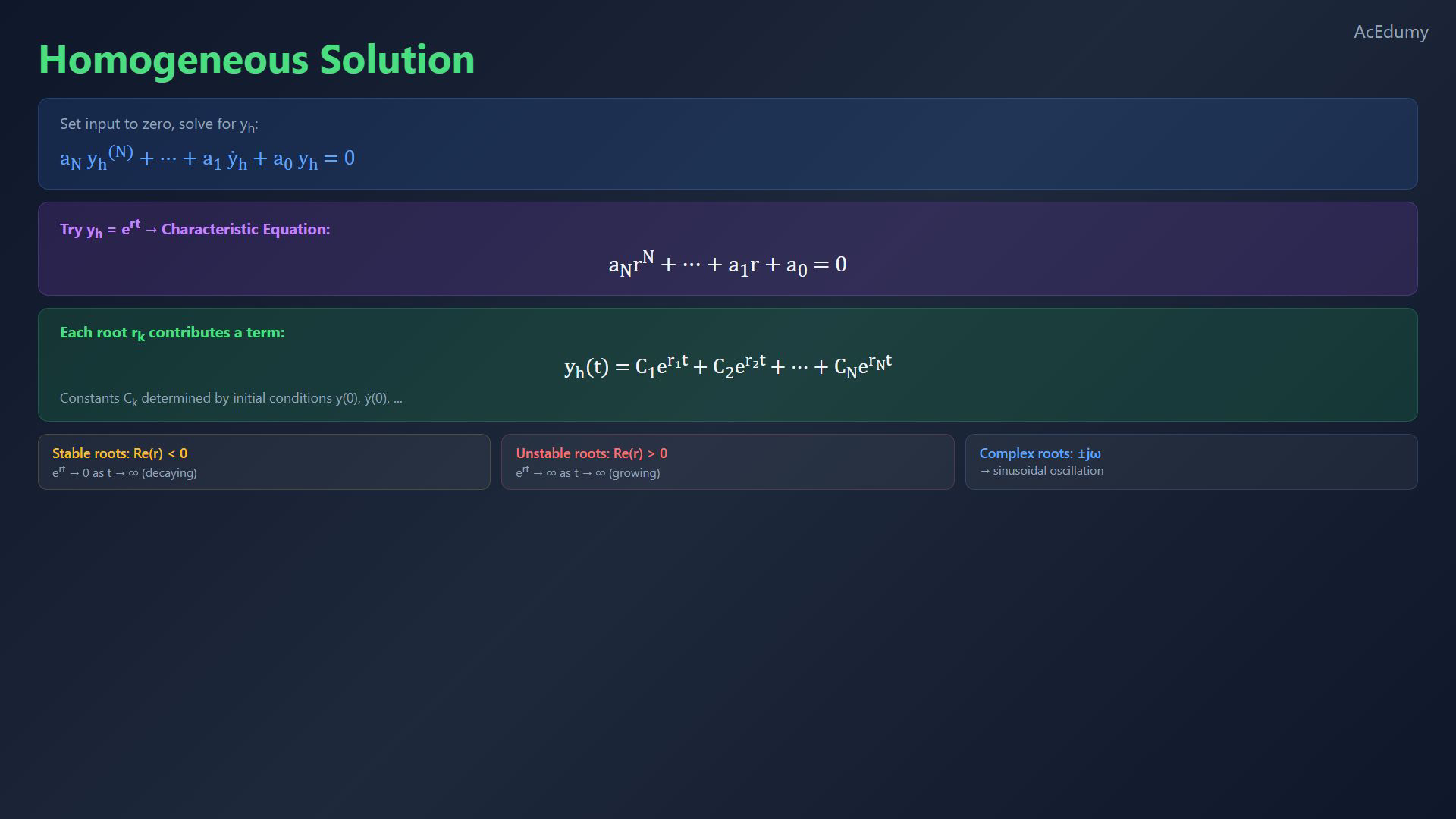
Original-video reference. The CT example shows the complete solution for a smooth exponential input. For the DT computation step, the reference is the general recursion card; the timed written lines give the three computed values. Read the simple-root and nonresonance assumptions in the problem statement.
Split the solution:
$\displaystyle y\left(t\right)=y_{h}\left(t\right)+y_{p}\left(t\right)$
Set the forcing to zero:
$\displaystyle \sum _{k=0}^{N}a_{k} y_{h}^{(k)}\left(t\right)=0$
Exponential trial gives the characteristic equation:
$\displaystyle a_{N} r^{N}+⋯+a_{1} r+a_{0}=0$
For distinct roots, each root contributes an exponential term.
Two distinct roots:
$\displaystyle y_{h}\left(t\right)=C_{1} e^{r_1 t}+C_{2} e^{r_2 t}$
Narration transcript
To solve the differential equation, we split the solution into two parts: y equals y h plus y p. The homogeneous solution y h satisfies the equation with the input set to zero. We try y h equals e to the r t, substitute into the left side, and extract the characteristic equation: a N times r to the N, plus dot dot dot, plus a one times r, plus a zero, equals zero. Each root r k gives a term C k times e to the r k t. For a second-order system with two distinct roots r one and r two, the homogeneous solution is: C one times e to the r one t, plus C two times e to the r two t — with constants determined by initial conditions.
3. Choose a particular solution
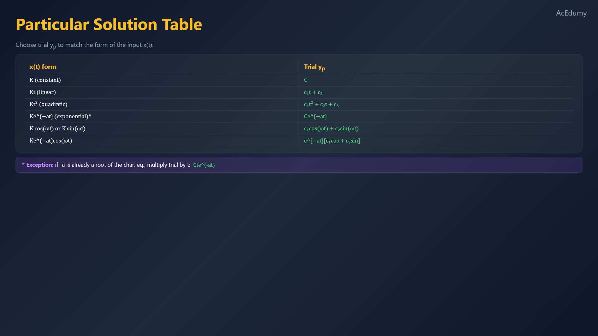
Original-video reference. The CT example shows the complete solution for a smooth exponential input. For the DT computation step, the reference is the general recursion card; the timed written lines give the three computed values. Read the simple-root and nonresonance assumptions in the problem statement.
Choose the particular trial from the forcing form, under the stated nonresonance conditions.
Constant forcing, when zero is not a root:
$\displaystyle y_{p}\left(t\right)=C$
Linear forcing, when zero is not a root:
$\displaystyle y_{p}\left(t\right)=c_{1} t+c_{2}$
If negative a is not a characteristic root:
$\displaystyle y_{p}\left(t\right)=C e^{-a t}$
Nonresonant sinusoidal forcing:
$\displaystyle y_{p}\left(t\right)=c_{1} \cos \left(\omega t\right)+c_{2} \sin \left(\omega t\right)$
Substitute into the full equation, collect terms, and solve for the constants.
Narration transcript
The particular solution y p matches the form of the forcing input. We choose a trial function from this table: if x is a constant K, try y p equals C. If x is linear in t, try c one t plus c two. If x is exponential, e to the negative a t, try capital C times e to the negative a t — but only when negative a is not already a root of the characteristic equation. For sinusoidal inputs of cosine omega t, try c one cosine omega t plus c two sine omega t. Substitute y p into the full equation, collect terms, and solve for the unknown constants.
4. Solve the CT example
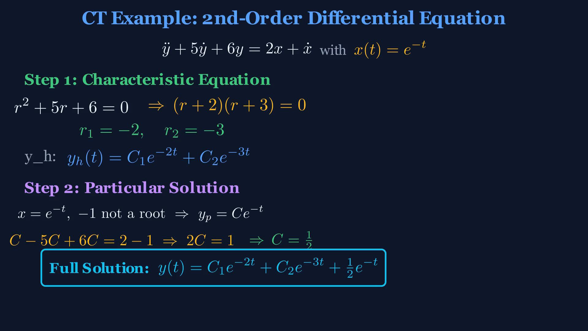
Original-video reference. The CT example shows the complete solution for a smooth exponential input. For the DT computation step, the reference is the general recursion card; the timed written lines give the three computed values. Read the simple-root and nonresonance assumptions in the problem statement.
Solve a second-order CT example.
Given equation:
$\displaystyle y''\left(t\right)+5y'\left(t\right)+6y\left(t\right)=2x\left(t\right)+x'\left(t\right)$
Smooth input:
$\displaystyle x\left(t\right)=e^{-t}$
Characteristic equation:
$\displaystyle r^{2}+5r+6=0$
Factor and find the roots:
$\displaystyle \left(r+2\right)\left(r+3\right)=0, r_{1}=-2, r_{2}=-3$
Homogeneous solution:
$\displaystyle y_{h}\left(t\right)=C_{1} e^{-2t}+C_{2} e^{-3t}$
Negative one is not a root, so try:
$\displaystyle y_{p}\left(t\right)=C e^{-t}$
Match coefficients:
$\displaystyle C-5C+6C=2-1, 2C=1, C=\frac{1}{2}$
Full solution:
$\displaystyle y\left(t\right)=C_{1} e^{-2t}+C_{2} e^{-3t}+\left(\frac{1}{2}\right)e^{-t}$
Apply the initial conditions to the full solution to determine both constants.
Narration transcript
Let's walk through a complete example. The differential equation is: the second derivative of y, plus 5 times the first derivative of y, plus 6 y, equals 2 x plus the first derivative of x. The input is x of t equals e to the negative t. First, the characteristic equation: r squared plus 5 r plus 6 equals zero. This factors as r plus 2, times r plus 3, giving roots r one equals negative 2, and r two equals negative 3. The homogeneous solution is C one times e to the negative 2 t, plus C two times e to the negative 3 t. For the particular solution, since x equals e to the negative t and negative 1 is not a root, we try y p equals capital C times e to the negative t. Substituting: C minus 5 C plus 6 C equals 2 minus 1, so 2 C equals 1 and C equals one half. The full solution is: y of t equals C one e to the negative 2 t, plus C two e to the negative 3 t, plus one half e to the negative t. The constants C one and C two are determined by initial conditions.
5. DT difference equations
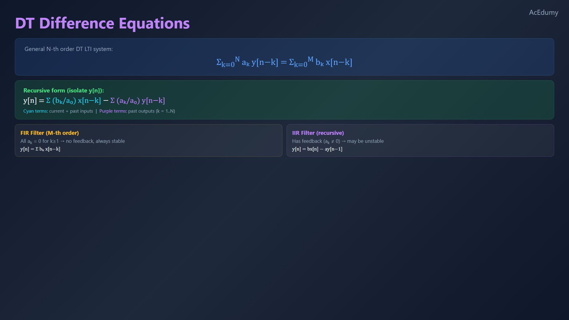
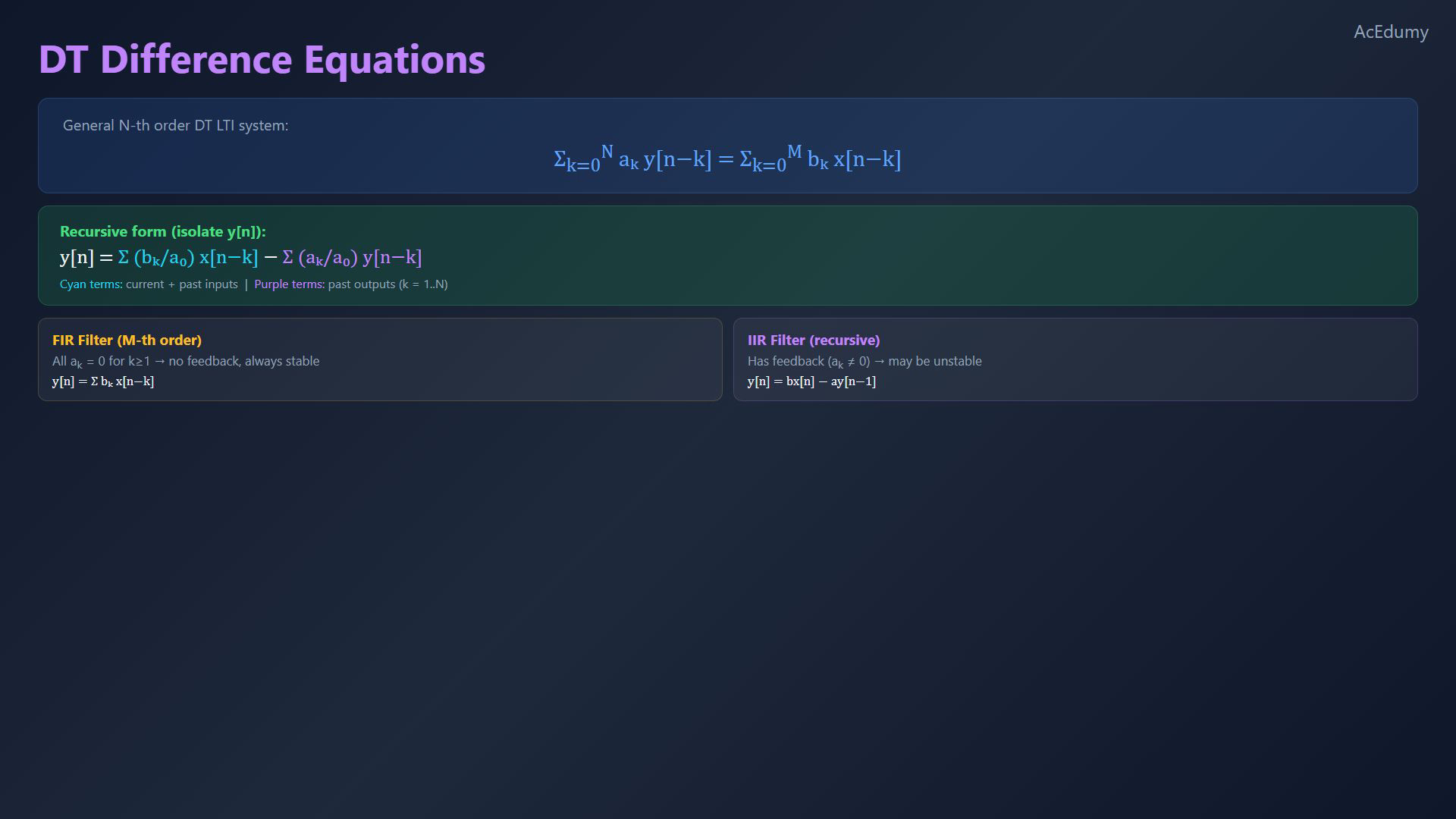
Original-video reference. The CT example shows the complete solution for a smooth exponential input. For the DT computation step, the reference is the general recursion card; the timed written lines give the three computed values. Read the simple-root and nonresonance assumptions in the problem statement.
Describe a DT system with a difference equation.
Constant-coefficient equation:
$\displaystyle \sum _{k=0}^{N}a_{k} y\left[n-k\right]=\sum _{k=0}^{M}b_{k} x\left[n-k\right]$
For nonzero leading coefficient:
$\displaystyle y\left[n\right]=\sum _{k=0}^{M}\left(\frac{b_{k}}{a_{0}}\right)x\left[n-k\right]-\sum _{k=1}^{N}\left(\frac{a_{k}}{a_{0}}\right)y\left[n-k\right]$
Compute each output from the input sequence and known past outputs.
Narration transcript
Discrete-time LTI systems are described by difference equations. The general form is: sum from k equals zero to N of a sub k times y of n minus k, equals sum from k equals zero to M of b sub k times x of n minus k. Dividing by a zero and isolating y of n gives a recursive formula: y of n equals the weighted sum of current and past inputs, minus the weighted sum of past outputs. This lets us compute each new output sample step by step, given the input sequence and initial conditions — this is exactly how digital filters work in practice.
6. Compute the DT example
Original-video reference. The CT example shows the complete solution for a smooth exponential input. For the DT computation step, the reference is the general recursion card; the timed written lines give the three computed values. Read the simple-root and nonresonance assumptions in the problem statement.
Given DT equation:
$\displaystyle y\left[n\right]+\left(\frac{1}{4}\right)y\left[n-1\right]=x\left[n\right]+2x\left[n-2\right]$
Unit-step input and zero initial output:
$\displaystyle x\left[n\right]=u\left[n\right], y\left[-1\right]=0$
Rearrange:
$\displaystyle y\left[n\right]=x\left[n\right]+2x\left[n-2\right]-\left(\frac{1}{4}\right)y\left[n-1\right]$
At index zero:
$\displaystyle y\left[0\right]=x\left[0\right]+2x\left[-2\right]-\left(\frac{1}{4}\right)y\left[-1\right]$
First output:
$\displaystyle y\left[0\right]=1+0-0=1$
At index one:
$\displaystyle y\left[1\right]=1+0-\left(\frac{1}{4}\right)1=\frac{3}{4}$
At index two:
$\displaystyle y\left[2\right]=1+2\left(1\right)-\left(\frac{1}{4}\right)\left(\frac{3}{4}\right)$
Third output:
$\displaystyle y\left[2\right]=3-\frac{3}{16}=\frac{45}{16}$
Each step uses current and past inputs plus past outputs.
Narration transcript
Let's compute the output for the system: y of n plus one quarter y of n minus one, equals x of n plus 2 times x of n minus two. The input is x of n equals the unit step u of n, with zero initial conditions. Rearranging: y of n equals x of n plus 2 times x of n minus two, minus one quarter times y of n minus one. At n equals zero: y zero equals x zero plus 2 times x of negative two, minus one quarter times y of negative one. That gives 1 plus 0 minus 0, equals 1. At n equals one: y one equals 1 plus 0 minus one quarter times 1, equals three fourths. At n equals two: y two equals 1 plus 2 times 1, minus one quarter times three fourths. That's 3 minus 3 over 16, giving 45 over 16. Each step uses the current input, past inputs, and past outputs.
7. Summary
Original-video reference. The CT example shows the complete solution for a smooth exponential input. For the DT computation step, the reference is the general recursion card; the timed written lines give the three computed values. Read the simple-root and nonresonance assumptions in the problem statement.
Solve the CT equation using a homogeneous part and a suitable particular trial.
Apply initial conditions to the full solution:
$\displaystyle y\left(t\right)=y_{h}\left(t\right)+y_{p}\left(t\right)$
DT difference equations yield recursive output computation.
The equation and initial conditions determine the response for an admissible input.
Next: relate impulse response and step response.
Narration transcript
Today we saw that continuous-time LTI systems are modeled by differential equations and solved in two stages: the homogeneous solution from the characteristic equation, and the particular solution matched to the input form. The full solution is y equals y h plus y p, with constants set by initial conditions. For discrete-time systems, difference equations lead to recursive computation — each output sample depends on past outputs and current and past inputs. Both approaches capture the same fundamental idea: the structure of the equation determines how the system responds to any input. In the next lesson, we'll connect this to the impulse response and step response.