#19 Zero-state LTI input-output maps, causal RC low-pass response, convolution and poles

Below are all the lines written in the notebook together with the full narration transcript.

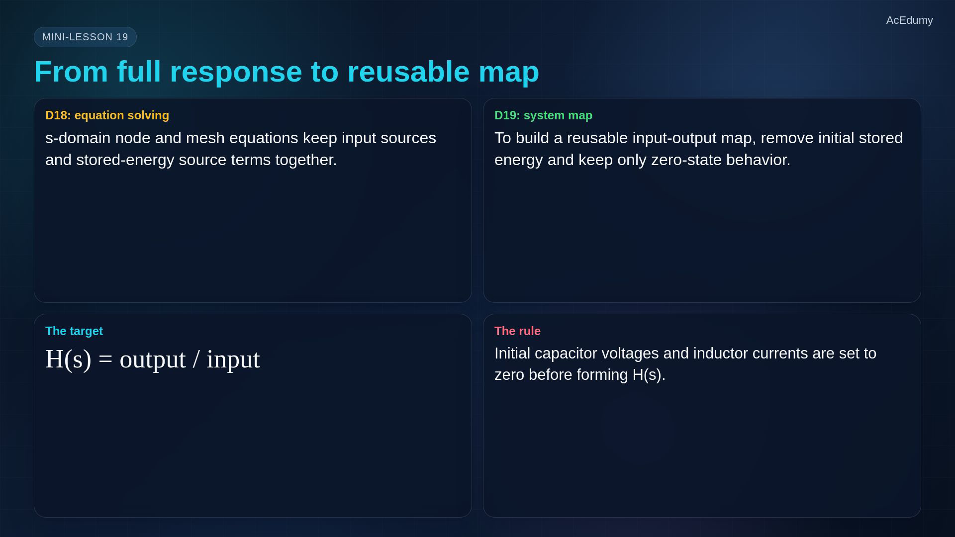
1. 1. Separate the zero-state system from the full response

   

   Lesson 18 combined the applied input and initial stored energy in s-domain equations.

   The complete response can include a zero-input part from the initial state.

   Now separate the input-output property of a linear time-invariant circuit.

   Choose the input and output, including their reference directions.

   The transfer function describes that chosen zero-state input-output relation.

   Set all independent initial stored energy to zero; do not remove dependent-source laws.

   Narration transcript

   Last time we used node and mesh equations directly in the s-domain. That gave us the complete response, including source terms from initial stored energy. Today we ask a different question. If this is the input, and that is the output, what reusable map connects them? That map is the transfer function. The price of getting a clean map is simple but important: all initial stored energy is set to zero.

2. 2. Define the input, output and transfer function

   

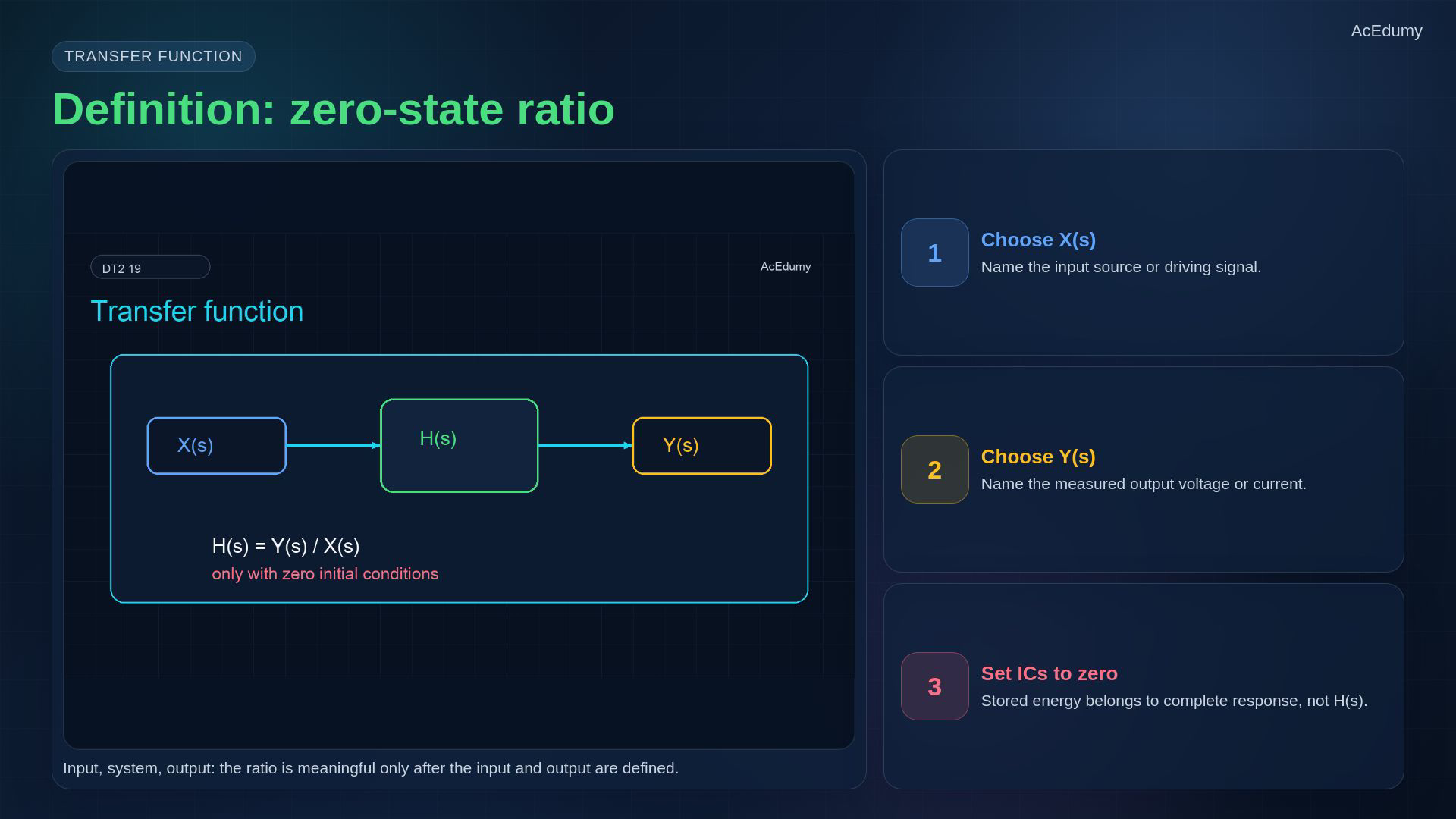
   For an LTI circuit with zero initial state:

   $\displaystyle H\left(s\right)=\frac{Y\left(s\right)}{X\left(s\right)}$

   X is the transform of the chosen input.

   Y is the transform of the chosen output.

   For a voltage input and capacitor-voltage output:

   $\displaystyle H\left(s\right)=\frac{V_{o}\left(s\right)}{V_{i}\left(s\right)}$

   A current output with a voltage input instead gives a transfer admittance, with units of siemens.

   The units and the input-output choice matter; a ratio alone is not enough.

   A transfer function excludes independent initial-state response terms.

   Narration transcript

   A transfer function is H of s equals Y of s divided by X of s, with zero initial conditions. X is the chosen input. Y is the chosen output. If the output is a capacitor voltage, H is a voltage ratio. If the output is a current, H can be current over voltage. So do not call every ratio a transfer function. It must be a zero-state input-output ratio.

3. 3. Write the RC low-pass input-output law

   

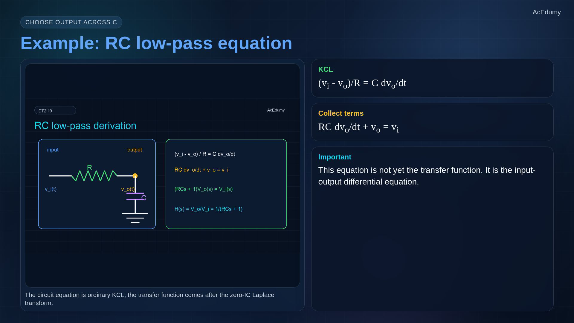
   Use ideal constant positive R and C in the RC low-pass circuit.

   The voltage input drives a series resistor; the capacitor connects the output node to the common reference.

   Measure both input and capacitor output voltages relative to that reference.

   KCL with passive branch currents:

   $\displaystyle \frac{v_{i}\left(t\right)-v_{o}\left(t\right)}{R}=\frac{C d v_{o}\left(t\right)}{\mathrm{d}t}$

   Collect the output terms:

   $\displaystyle \frac{R C d v_{o}\left(t\right)}{\mathrm{d}t}+v_{o}\left(t\right)=v_{i}\left(t\right)$

   Narration transcript

   Use the classic RC low-pass circuit. A source drives a series resistor, then a capacitor to ground. The output is the capacitor voltage. At the output node, the resistor current equals the capacitor current: V input minus V output, divided by R, equals C times d V output over d t. After collecting terms, R C times d V output over d t plus V output equals V input.

4. 4. Transform with zero initial capacitor voltage

   

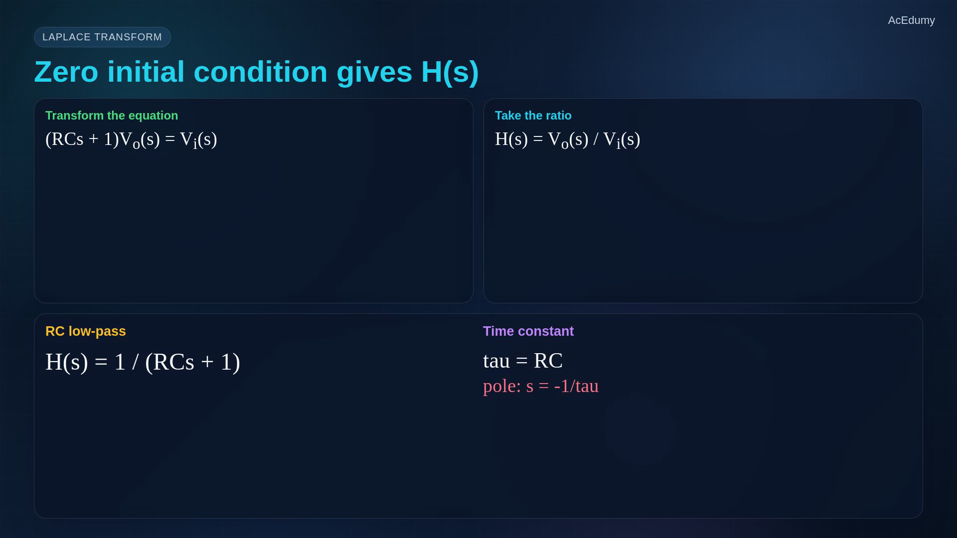
   Use the zero-minus unilateral convention and initially uncharged capacitor:

   $\displaystyle v_{o}\left(0^{-}\right)=0$

   The transformed derivative has no initial-voltage contribution:

   $\displaystyle D_{o}\left(s\right)=s V_{o}\left(s\right)$

   Transform the complete input-output equation:

   $\displaystyle \left(R C s+1\right)V_{o}\left(s\right)=V_{i}\left(s\right)$

   The voltage transfer function is dimensionless:

   $\displaystyle H\left(s\right)=\frac{V_{o}\left(s\right)}{V_{i}\left(s\right)}=\frac{1}{R C s+1}$

   The time constant is positive and the pole negative:

   $\displaystyle \tau =R C, H\left(s\right)=\frac{1}{\tau s+1}, p=-\frac{1}{\tau }$

   Narration transcript

   Now take the Laplace transform with zero initial capacitor voltage. The derivative becomes s times V output of s, with no extra initial-condition term. So open parenthesis R C s plus one close parenthesis V output equals V input. Therefore H of s equals V output over V input equals one over R C s plus one. If tau equals R C, then H of s is one over tau s plus one, with a pole at minus one over tau.

5. 5. Find the causal impulse response

   

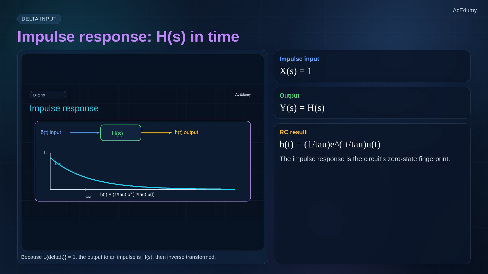
   Apply a normalized ideal impulse to this initially relaxed causal system:

   $\displaystyle x\left(t\right)=\delta \left(t\right)$

   The impulse transform is one:

   $\displaystyle X\left(s\right)=1, Y\left(s\right)=H\left(s\right)$

   Invert H with the causal region of convergence to obtain the impulse response.

   Use the positive decay rate for a readable exponent:

   $\displaystyle a=\frac{1}{\tau }, h\left(t\right)=a e^{-a t}u\left(t\right)$

   This is the zero-state impulse response; its right-limit jump does not imply a nonzero zero-minus initial state.

   Narration transcript

   Impulse response asks what comes out when the input is the ideal impulse delta of t. Because the Laplace transform of delta is one, the output in the s-domain is simply H of s. So the impulse response h of t is the inverse Laplace transform of H of s. For the RC low-pass, h of t equals one over tau times e to the minus t over tau, times u of t. It is the circuit's zero-state fingerprint.

6. 6. Reuse the impulse response for another input

   

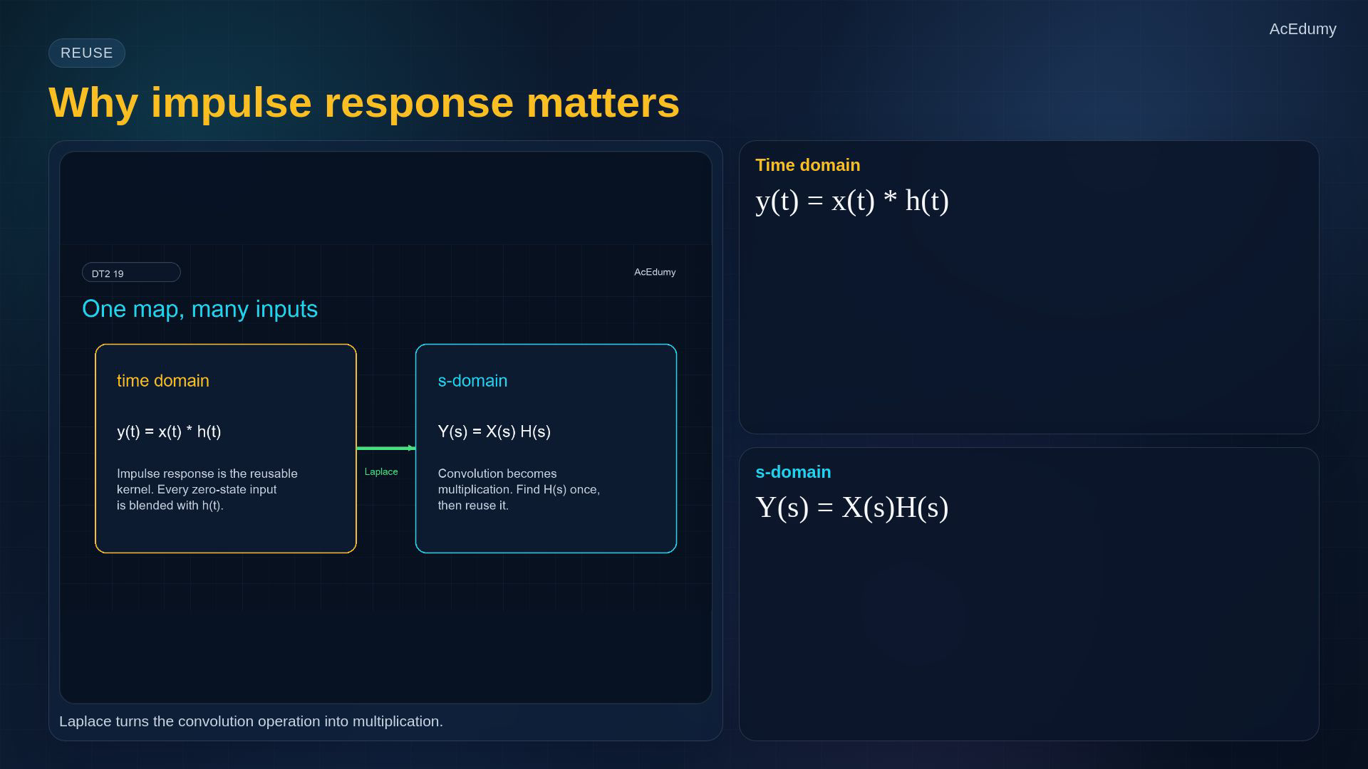
   Knowing one impulse response lets us calculate many zero-state responses.

   For causal ordinary inputs where the integral exists, convolution is:

   $\displaystyle y\left(t\right)=\int _{0}^{t} x\left(\xi \right) h\left(t-\xi \right) \mathrm{d}\xi$

   Convolution in time becomes ordinary multiplication in the common transform region:

   $\displaystyle Y\left(s\right)=X\left(s\right)H\left(s\right)$

   Do not replace the convolution integral by pointwise multiplication of the two time functions.

   The same LTI input-output map can be reused with another admissible input.

   Narration transcript

   Why is this powerful? Once we know h of t, every zero-state output can be written as a convolution: y of t equals x of t convolved with h of t. In the s-domain, that convolution becomes multiplication: Y of s equals X of s times H of s. So the transfer function is not just a formula. It is a reusable shortcut from input to output.

7. 7. Read the reduced RC transfer function

   

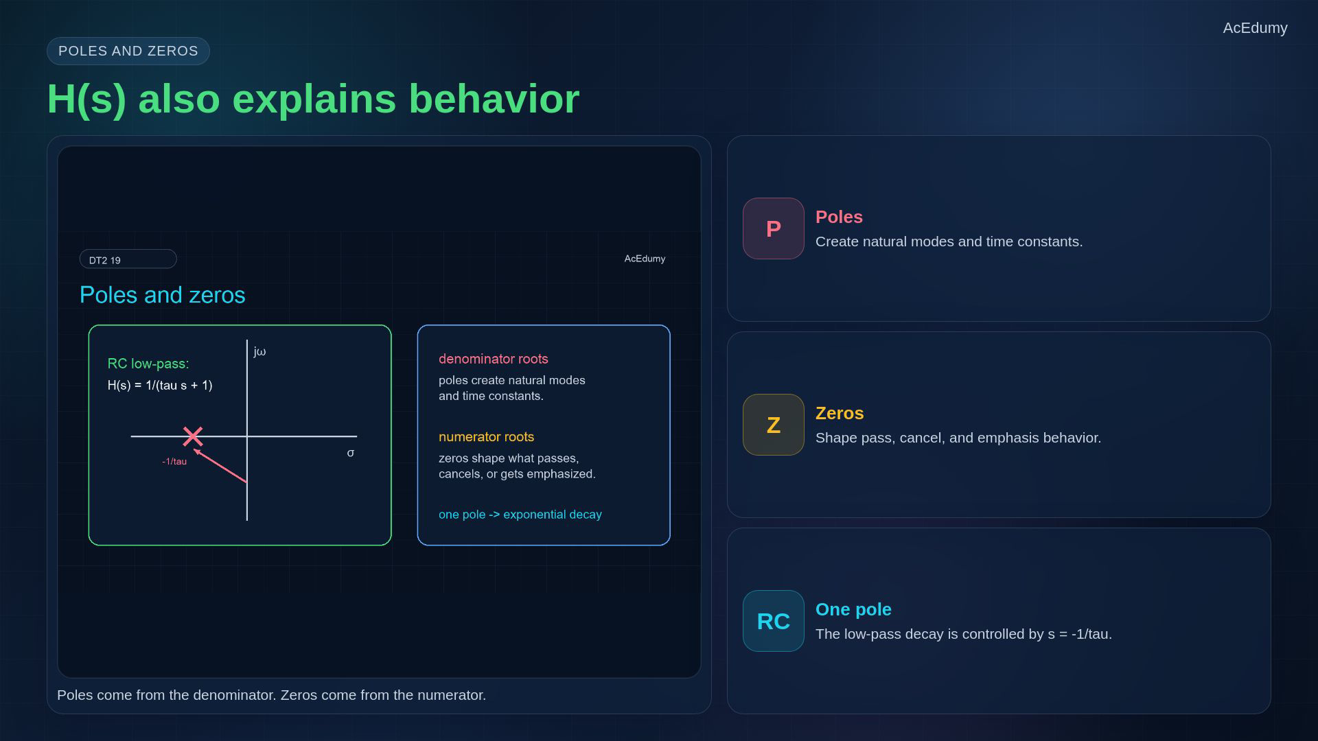
   Read poles and zeros from the reduced transfer function, with the input-output choice fixed.

   After cancelling common polynomial factors, denominator roots are the transfer poles.

   Numerator roots are transfer zeros; cancellations alone do not establish internal stability.

   For this positive RC circuit there is no finite zero and one pole:

   $\displaystyle H\left(s\right)=\frac{1}{\tau s+1}, p=-\frac{1}{\tau }$

   Its causal mode decays, and the RC low-pass magnitude tends to zero at high frequency.

   Narration transcript

   The same H of s also explains behavior. Denominator roots are poles, and they create natural modes. Numerator roots are zeros, and they shape which parts of the input pass, cancel, or get emphasized. For the RC low-pass, there is no finite zero and one pole at minus one over tau. That single pole gives the exponential decay and the high-frequency attenuation.

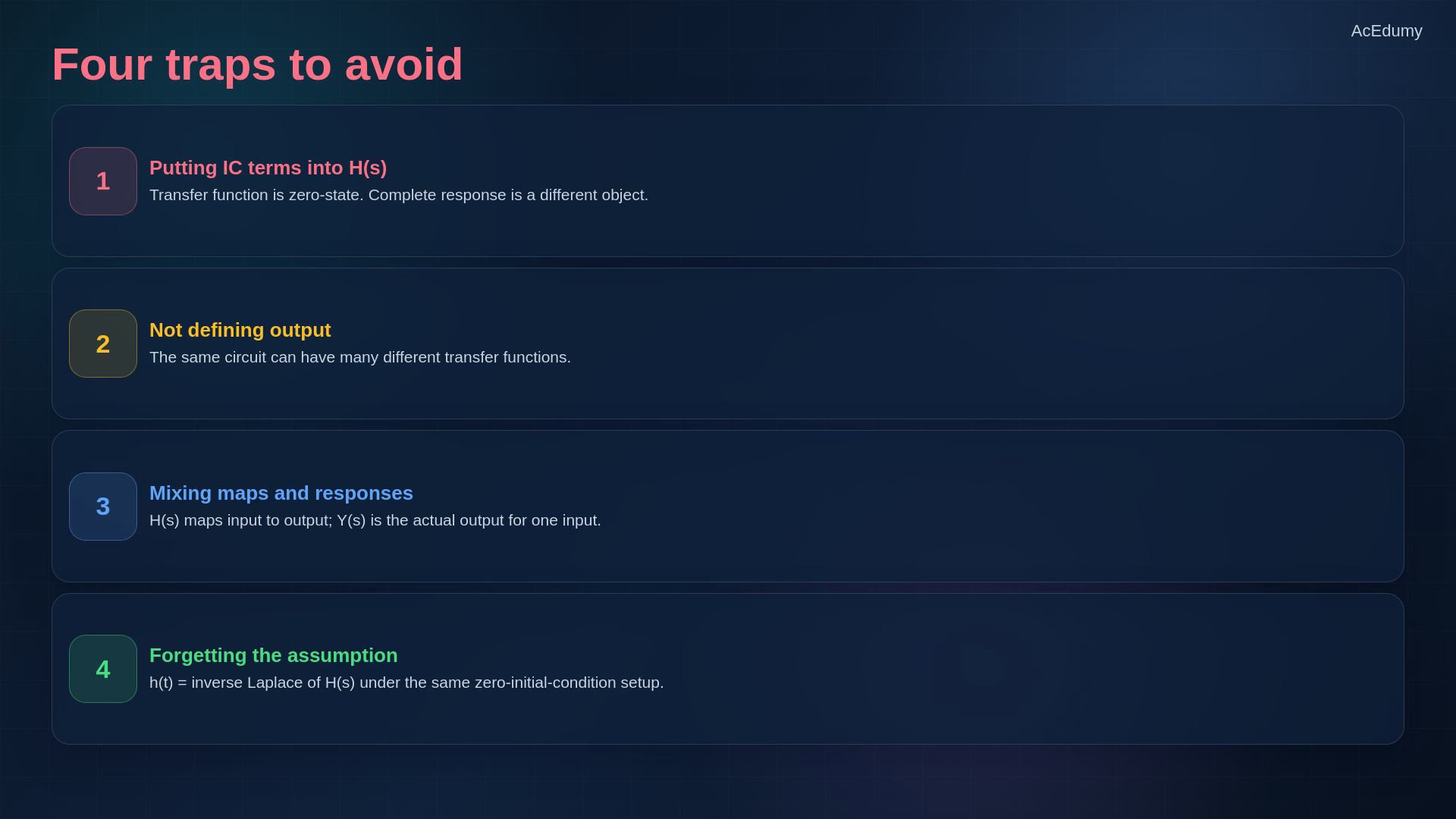
8. 8. Keep the input-output and initial-state assumptions

   

   Four assumptions to keep visible.

   Exclude independent initial-condition source terms from the transfer function.

   State both the input and output: different choices can give different ratios and units.

   Do not confuse the complete response with its zero-state input-output map.

   The impulse response uses the same initially relaxed LTI system and the appropriate causal transform region.

   Narration transcript

   Four traps are worth naming. First, do not include initial-condition source terms inside the transfer function. Second, always state both the input and the output, because changing the output changes H of s. Third, do not mix the complete response with the zero-state map. Fourth, remember that impulse response is the inverse transform of H only under the same zero-initial-condition assumption.

9. 9. Connect transfer function, impulse response and convolution

   

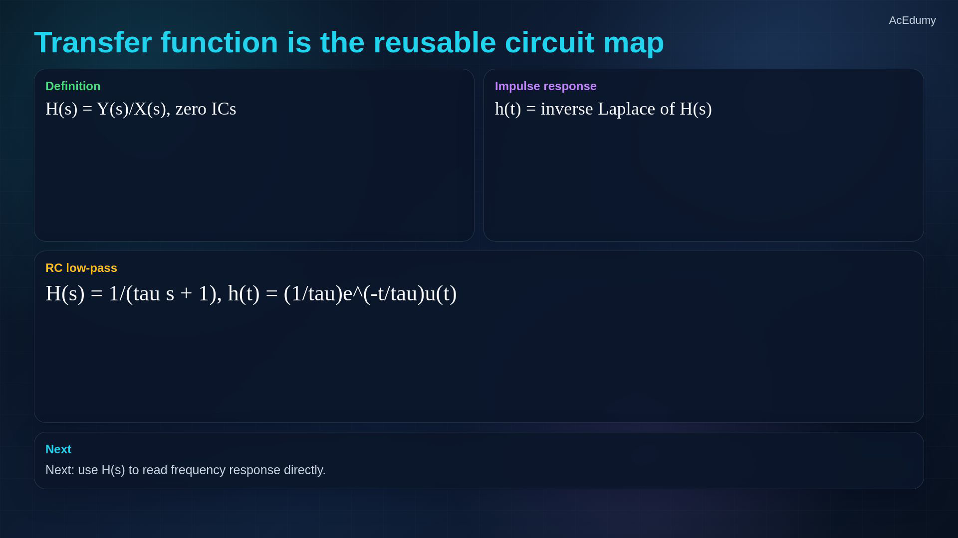
   Summary: one circuit description, two equivalent domains.

   With zero initial state and the chosen input-output pair:

   $\displaystyle H\left(s\right)=\frac{Y\left(s\right)}{X\left(s\right)}$

   For the RC voltage low-pass:

   $\displaystyle \tau =R C, H\left(s\right)=\frac{1}{\tau s+1}$

   Its causal inverse transform is the impulse response:

   $\displaystyle a=\frac{1}{\tau }, h\left(t\right)=a e^{-a t}u\left(t\right)$

   For admissible inputs, obtain the zero-state response by convolution; add any independent initial-state response separately.

   Next: for this stable causal RC system, evaluate the transfer function on the imaginary axis to study frequency response.

   Narration transcript

   Summary. A transfer function is the zero-state ratio Y of s over X of s. For the RC low-pass, H of s equals one over tau s plus one. The impulse response is the time-domain version of that map: h of t equals the inverse Laplace transform of H of s. And for any input, zero-state output is input convolved with impulse response. Next, we use H of s to read frequency behavior directly.

Source video: Circuit Theory-2 #19 | Transfer Function and Impulse Response (4:45)