Circuit Theory 2 · Two-port networks: h and ABCD parameters

#28 Hybrid test conditions, transmission signs, ordered cascades and source/load transformations

Use hybrid test conditions and a consistent transmission-current sign to calculate cascades, input impedance and loaded voltage transfer.

Question

Reviewed same-video reference on hybrid parameters, two-port model choice and ordered cascades. — Original-video reference; three diagram roles use reviewed overview or summary frames. Explicit equations, test conditions and port signs are provided in the notebook.

Consider an initially relaxed linear time-invariant two-port, or an incremental model about a stated bias, within its linear operating range and with independent-source offsets appropriately removed. Each terminal pair must satisfy the port condition: entering current returns through its paired terminal. V1,V2 are upper-minus-lower voltages; I1,I2 enter the upper positive-reference terminals. Parameters may depend on frequency or Laplace variable. Choose a finite representation only where independent variables determine unique dependent variables. Hybrid form uses independent I1,V2 and dependent V1,I2: V1=h11I1+h12V2,I2=h21I1+h22V2. Units in row order are ohms,dimensionless,dimensionless,siemens. With V2=0 and nonzero I1,h11=V1/I1,h21=I2/I1. With I1=0 and nonzero V2,h12=V1/V2,h22=I2/V2. The source phrase read from the port-one or port-two side names the driven test port, not the location of every measured variable: V1 and I2 are measured in both tests. A short sets voltage zero, not current; an open sets current zero, not voltage. Test-specific input impedance/current ratio labels are not arbitrary loaded gains. The outward load current is IL=−I2, so short-output load-current gain is −h21. Transistor h models need bias, frequency range and small-signal approximation; no arbitrary nonlinear large-signal prediction. Where z exists with z22 nonzero, ΔZ=z11z22−z12z21 and h11=ΔZ/z22,h12=z12/z22,h21=−z21/z22,h22=1/z22. Reciprocity gives h12=−h21, not equality with these current references. Transmission form defines J2=−I2: [V1;I1]=M[V2;J2] with M=[[A,B],[C,D]], so V1=AV2+BJ2 and I1=CV2+DJ2. These are column vectors; the source raster horizontal bracket shorthand is not a valid row-vector product. A,D dimensionless,B ohms,C siemens. A=V1/V2 and C=I1/V2 only with J2=0 (output open); B=V1/J2 and D=I1/J2 only with V2=0 (output short), with valid nonzero denominators. For physical stage1→stage2→stage3 cascade, consistent entering references give upstream J2 equal to next I1 and joined port voltages equal. Thus Mtotal=M1M2M3, generally not reversed or commutative. Model validity, preserved port conditions and no extra cross-coupling between blocks are required. Correct transmission matrices include modeled interstage loading; a buffer is not intrinsically required. Ideal seriesZ gives [[1,Z],[0,1]], shuntY gives [[1,0],[Y,1]]; series-then-shunt gives [[1+ZY,Z],[Y,1]], shunt-then-series gives [[1,Z],[Y,1+YZ]]. For finite nonzero ZL with J2=V2/ZL,Zin=V1/I1=(AZL+B)/(CZL+D) when well-defined. V2/V1=1/(A+B/ZL); with Thevenin Vs=V1+ZsI1,V2/Vs=ZL/[AZL+B+Zs(CZL+D)]. The killed-independent-source output impedance is Zout=(B+ZsD)/(A+ZsC), with input termination V1=−ZsI1 and a valid test denominator. Source/load effects are not galvanic isolation or inevitable load dependence for every ideal active model. At fixed ABCD,dZin/dZL=(AD−BC)/(CZL+D)^2; a determinant-zero unilateral model can have load-independent input impedance. Output-open Zin=A/C if finite; output-short Zin=B/D if finite. Handle zero/infinite impedances as proper limits; never cancel0/0 or divide by a singular coefficient. Not every circuit has all representations at every frequency. Where finite z exists and z21≠0,A=z11/z21,B=ΔZ/z21,C=1/z21,D=z22/z21;detM=z12/z21. Reciprocity gives detM=1 where it exists, not a universal active/nonreciprocal rule. Where h21≠0,A=h12−h11h22/h21,B=−h11/h21,C=−h22/h21,D=−1/h21. Passive resistive T arms2Ω/3Ω,shunt5Ω givesZ=[[7,5],[5,8]],Δ31,H=[[31/8,5/8],[−5/8,1/8]],M=[[7/5,31/5],[1/5,8/5]]. RL4Ω givesZin59/12Ω,V2/V1=20/59;sourceRs2Ω givesV2/Vs20/83. Killed-source output resistance also follows direct reduction3+(5||4)=47/9Ω. A known termination alone normally cannot identify four independent coefficients; use sufficiently independent equations, existence and conditioning checks. Open/short tests may be analytical or simulated; do not physically short a powered amplifier without device-safe procedures. Practical toolbox is not exhaustive: inverse-hybrid/scattering and other representations also exist. All117audio-source/356TSX/443graph lines and EN metadata read, SCENES AST only, no source generators run. Original final243.264000s/20,141,828bytes,SHA33dda0354d8ffcd87640229be8c07d5d921a2c12ea6617554a44f44b5aa8dced and9MP3+timings11sourceSHA equal readonly Hetzner. MP3/final correlations.96773–.98223,27–55ms. Cached-large ASR all9passages/39cue intervals read; common English closed-vocabulary normalization fixes compact h11/h21 and V1/I1 spelling without threshold/narration/source change. Final confidence.9951–1. Independent cached-small original MP3 and matching final86.943–110.863s,191.11–216.31s recognize negativeI2 and known load correctly. Large-ASR extra the/non-load is not established wrong source speech; no manual word-time override or full human listening claim. All9final frames reviewed. abcd-definition→bridge avoids row-vector pseudo-matrix and covered voltage labels;terminated→summary avoids load leads20sourcepixels off actual port terminals;choose-model→bridge avoids footer box/text overflow. Six unique same-final references across9roles; no repaint/newrender/motion validation. Retained h definitions/ratios readable with explicit tests; cascade is conceptual with stage-specific matrices and physical order; workflow/summary clear. Original9MP3/say/39cue boundaries preserved; displayed equations and scope clarified only. Technical unpublished draft; no TTS/paidgeneration/modeldownload/video render/upload/publication/access/security/egress changes; human teaching/motion/publication QA outstanding.

Written solution and narration transcript(shows the full solution)

Below are all the lines written in the notebook together with the full narration transcript.

1. Choose another valid two-port representation
Original-video reference; three diagram roles use reviewed overview or summary frames. Explicit equations, test conditions and port signs are provided in the notebook.
Use another coordinate choice for the same linear two-port.
Keep the port references and operating conditions when changing parameter models.
A representation is usable only where its independent variables give a finite, unique response.
Hybrid form mixes current and voltage; transmission form is convenient for properly connected cascades.
Narration transcript
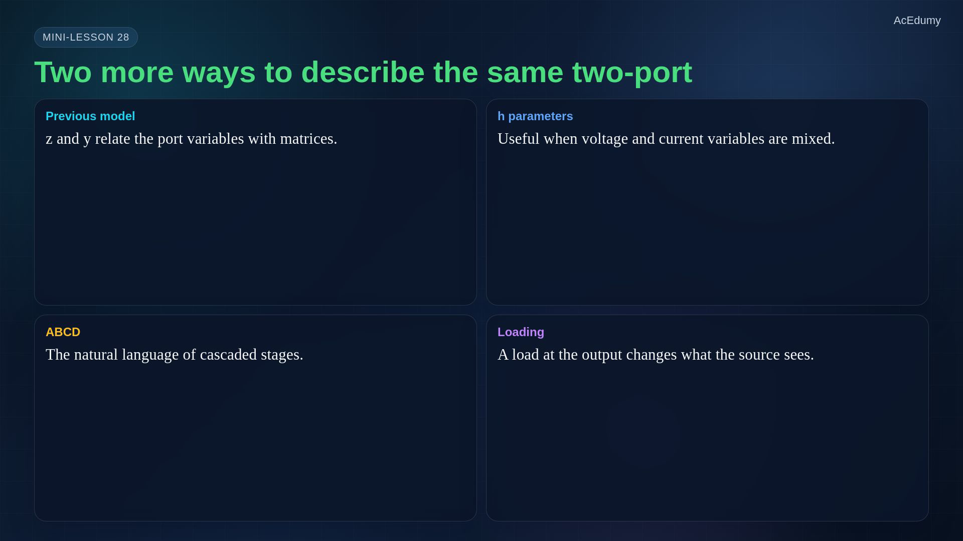
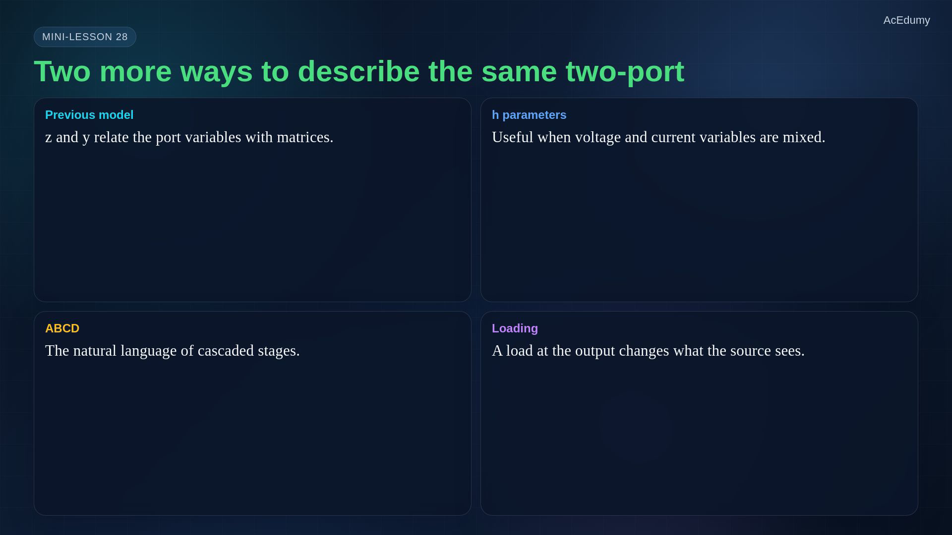
In the previous lesson, we described a two-port with z parameters and y parameters. The idea was simple: choose port variables, then write a matrix that relates them. In this lesson we add two more models. h parameters are useful when voltages and currents are mixed, and ABCD parameters are especially useful when stages are connected in cascade.
2. State the hybrid equations and mixed units
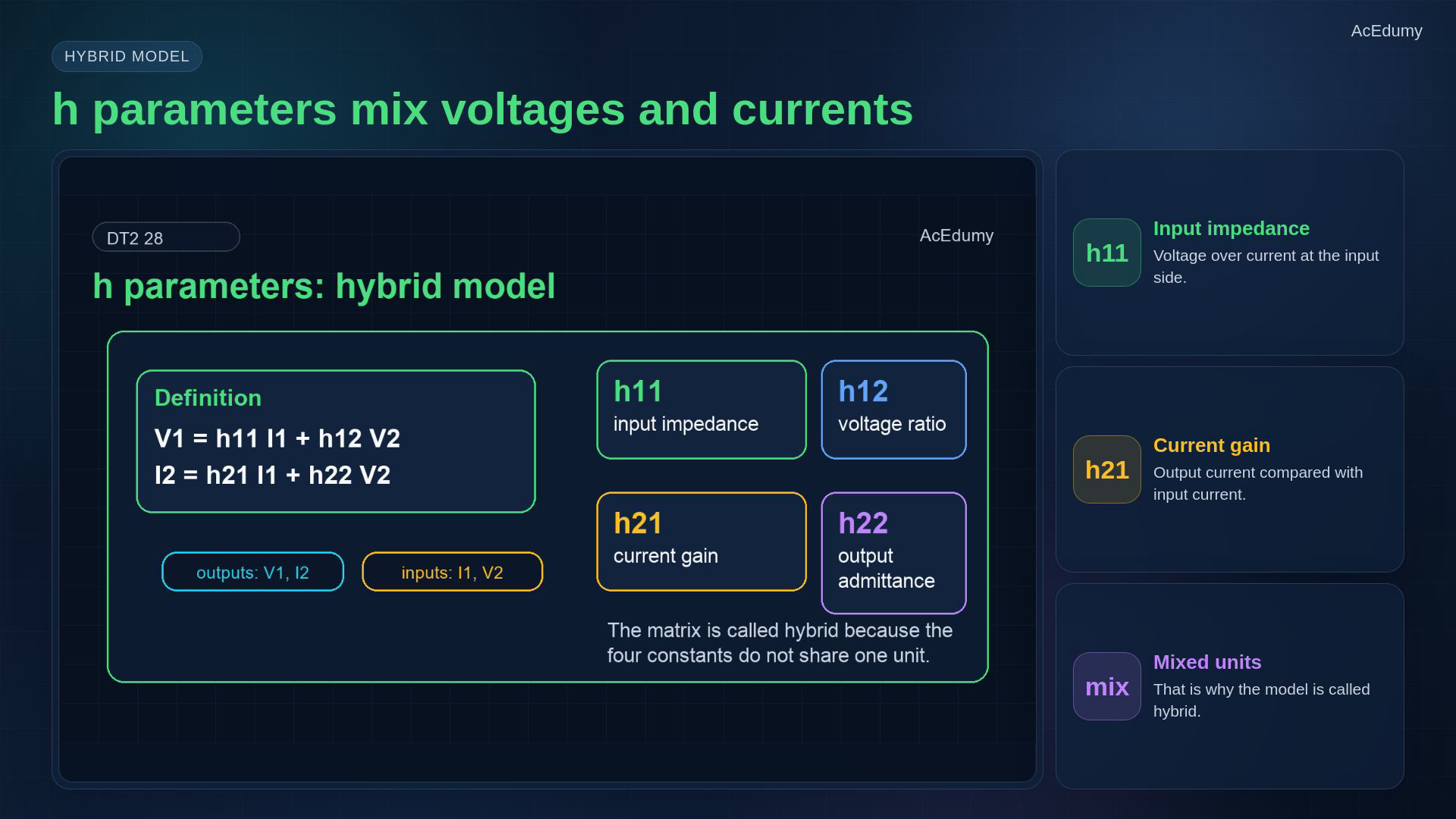
Original-video reference; three diagram roles use reviewed overview or summary frames. Explicit equations, test conditions and port signs are provided in the notebook.
Hybrid parameters describe input voltage and output current using input current and output voltage.
First hybrid equation:
$\displaystyle V_{1}=h_{11} I_{1}+h_{12} V_{2}$
Second hybrid equation:
$\displaystyle I_{2}=h_{21} I_{1}+h_{22} V_{2}$
The four units, in row order, are ohms, dimensionless, dimensionless and siemens. Transistor use assumes a stated small-signal bias.
Narration transcript
We start with h parameters, also called hybrid parameters. They are hybrid because the first equation gives the voltage at port one, while the second equation gives the current at port two. Inside the same matrix, the constants do not all have the same units: one behaves like an impedance, one like a voltage ratio, one like a current ratio, and one like an admittance. That is why this model is common in amplifier and transistor models.
3. Separate hybrid short-output and open-input tests
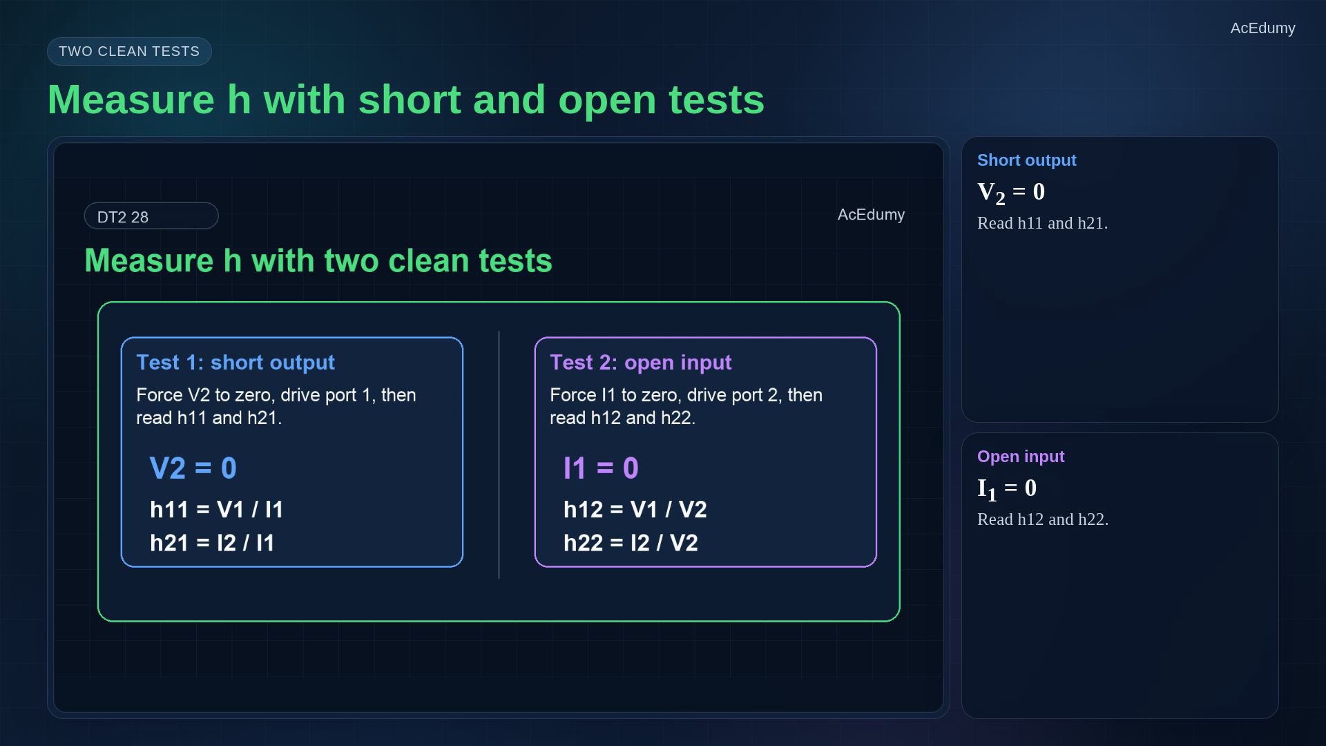
Original-video reference; three diagram roles use reviewed overview or summary frames. Explicit equations, test conditions and port signs are provided in the notebook.
Use the matching test conditions and nonzero driven variable to extract each hybrid column.
For the first test, short the output:
$\displaystyle V_{2}=0$
Drive port one; measure input voltage and output current:
$\displaystyle h_{11}=\frac{V_{1}}{I_{1}}, h_{21}=\frac{I_{2}}{I_{1}}$
For the second test, open the input:
$\displaystyle I_{1}=0$
Drive port two; measure input voltage and output current:
$\displaystyle h_{12}=\frac{V_{1}}{V_{2}}, h_{22}=\frac{I_{2}}{V_{2}}$
Narration transcript
To measure h parameters, use two clean tests. In the first test, set the output voltage to zero: short port two. Then h eleven and h twenty one are read from the port-one side. In the second test, set the input current to zero: open port one. Then h twelve and h twenty two are read from the port-two side.
4. Use the negative entering output current in transmission form
Original-video reference; three diagram roles use reviewed overview or summary frames. Explicit equations, test conditions and port signs are provided in the notebook.
Use a finite transmission representation with both port voltages measured upper to lower.
The input voltage depends on output voltage and outward output current:
$\displaystyle V_{1}=A V_{2}+B J_{2}$
The input current uses that same outward output current:
$\displaystyle I_{1}=C V_{2}+D J_{2}$
Both original port currents enter the network, so define the outward output current as:
$\displaystyle J_{2}=-I_{2}$
Narration transcript
Now switch to ABCD parameters. This is called the transmission model because it relates the input-side variables to the output-side variables. We write V one and I one in terms of V two and the output current. With the standard two-port convention, I two is defined entering the network, so the transmission form uses negative I two.
5. Multiply transmission matrices in physical order
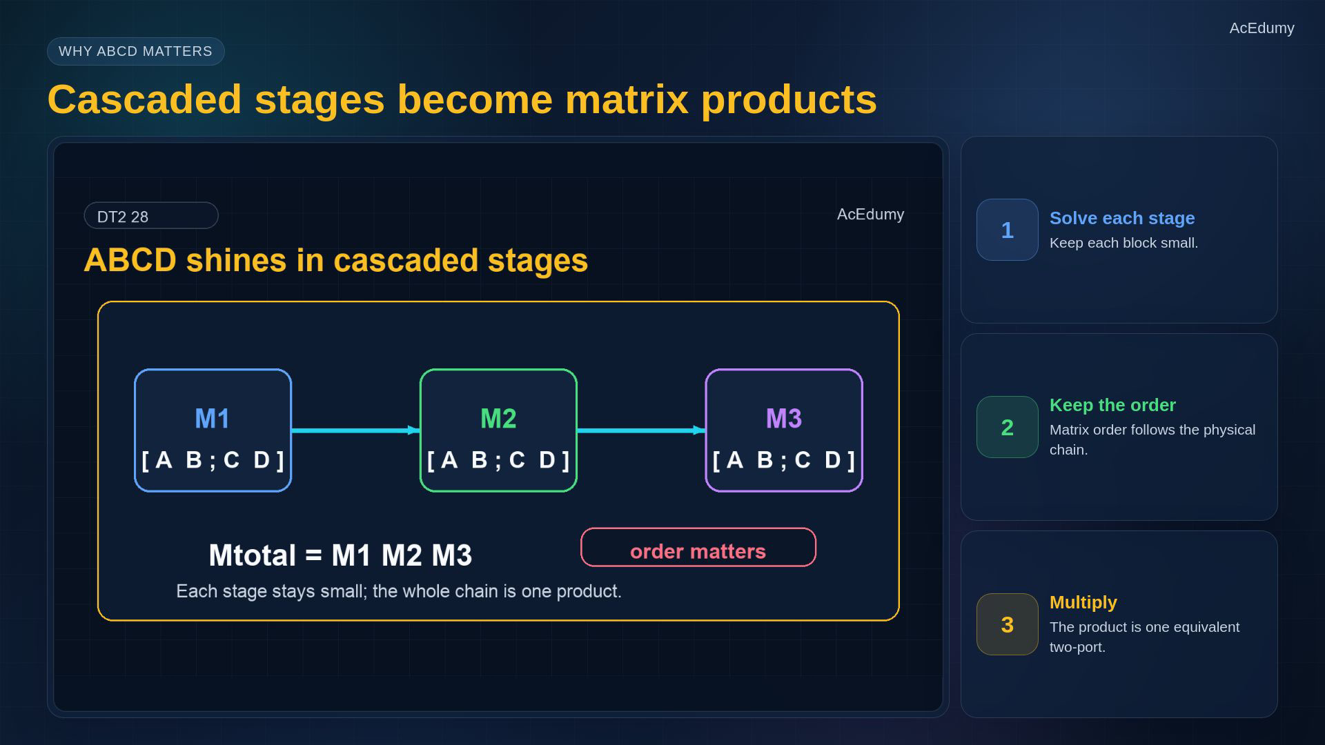
Original-video reference; three diagram roles use reviewed overview or summary frames. Explicit equations, test conditions and port signs are provided in the notebook.
A transmission matrix maps the output column vector to the input column vector.
Connect stage one to stage two, then stage three, preserving the port conditions and current signs.
Multiply in the physical input-to-output order:
$\displaystyle M=M_{1} M_{2} M_{3}$
Matrix multiplication is generally not commutative; a different order represents a different connection.
Narration transcript
The real power of ABCD parameters appears in cascaded stages. If stage one feeds stage two, and stage two feeds stage three, we do not reanalyze the whole circuit as one large object. We compute the matrix of each stage, then multiply the matrices in order. A large network becomes a chain of small steps.
6. Transform a valid termination to input impedance
Original-video reference; three diagram roles use reviewed overview or summary frames. Explicit equations, test conditions and port signs are provided in the notebook.
Assume a valid finite load and transmission model; load dependence is common, not universal for every ideal two-port.
The current delivered to the load is opposite the entering second-port current:
$\displaystyle V_{2}=Z_{L} J_{2}$
For a well-defined denominator, the source sees:
$\displaystyle Z_{\mathrm{in}}=\frac{A Z_{L}+B}{C Z_{L}+D}$
Including a Thevenin source impedance, the loaded voltage transfer is:
$\displaystyle \frac{V_{2}}{V_{s}}=\frac{Z_{L}}{A Z_{L}+B+Z_{s} \left(C Z_{L}+D\right)}$
Narration transcript
When a load is connected to the output, the load is not isolated anymore. The ABCD matrix transforms that load into an input impedance seen by the source. This lets us compute Zin from A, B, C, D, and the load value. The same idea also tells us that the source side affects what we see at the output.
7. Choose a parameter representation that exists
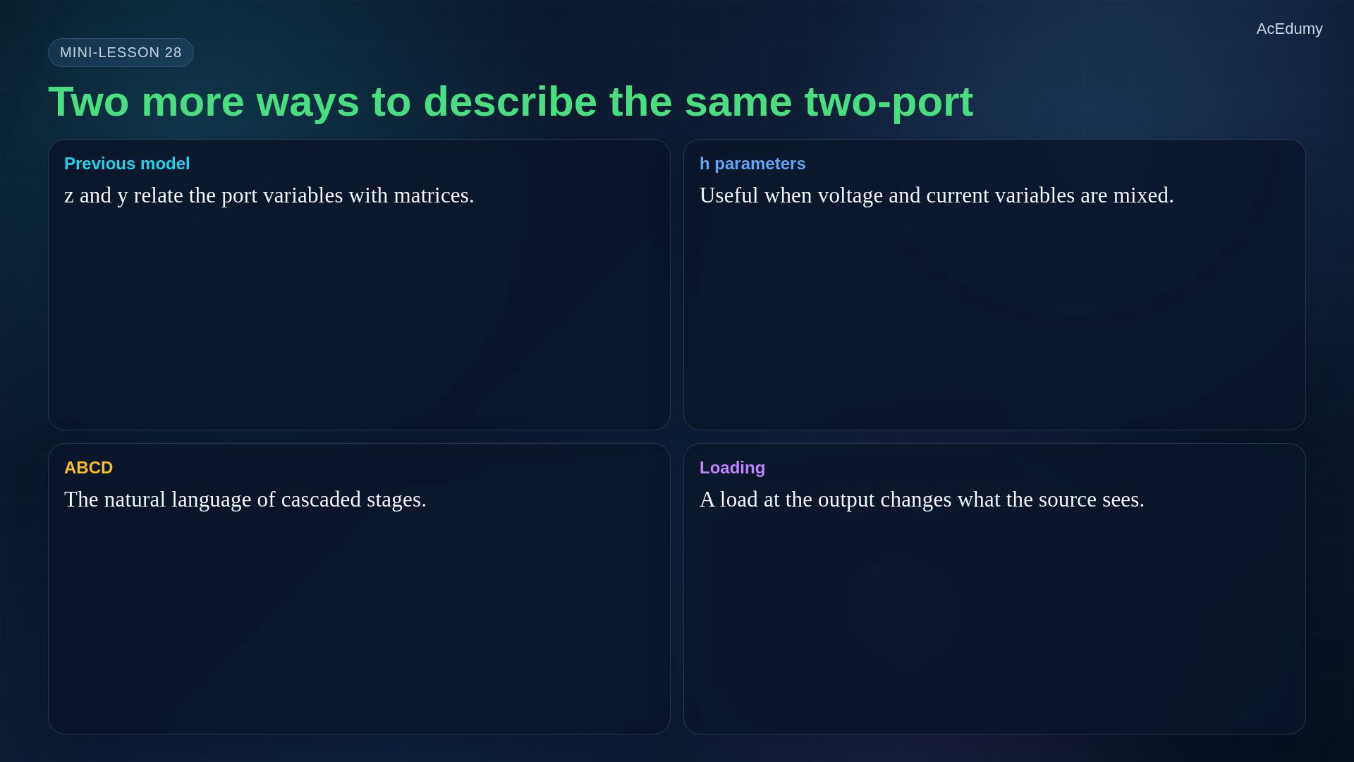
Original-video reference; three diagram roles use reviewed overview or summary frames. Explicit equations, test conditions and port signs are provided in the notebook.
Choose a convenient representation that actually exists at the operating point or frequency.
Impedance form is convenient for open-circuit tests and suitable series relations.
Admittance form is convenient for short-circuit tests and nodal relations.
Hybrid form uses mixed variables and is often useful for small-signal amplifier models.
Transmission form is convenient for cascades and terminated networks, with its output-current sign kept explicit.
Narration transcript
So which model should you choose? Use z parameters when open-circuit tests and impedances are natural. Use y parameters when short-circuit tests or nodal equations are cleaner. Use h parameters for amplifiers or transistor-style models with mixed input and output variables. Use ABCD parameters for cascaded stages, transmission lines, and loaded networks.
8. Verify conventions, conditions and loaded response
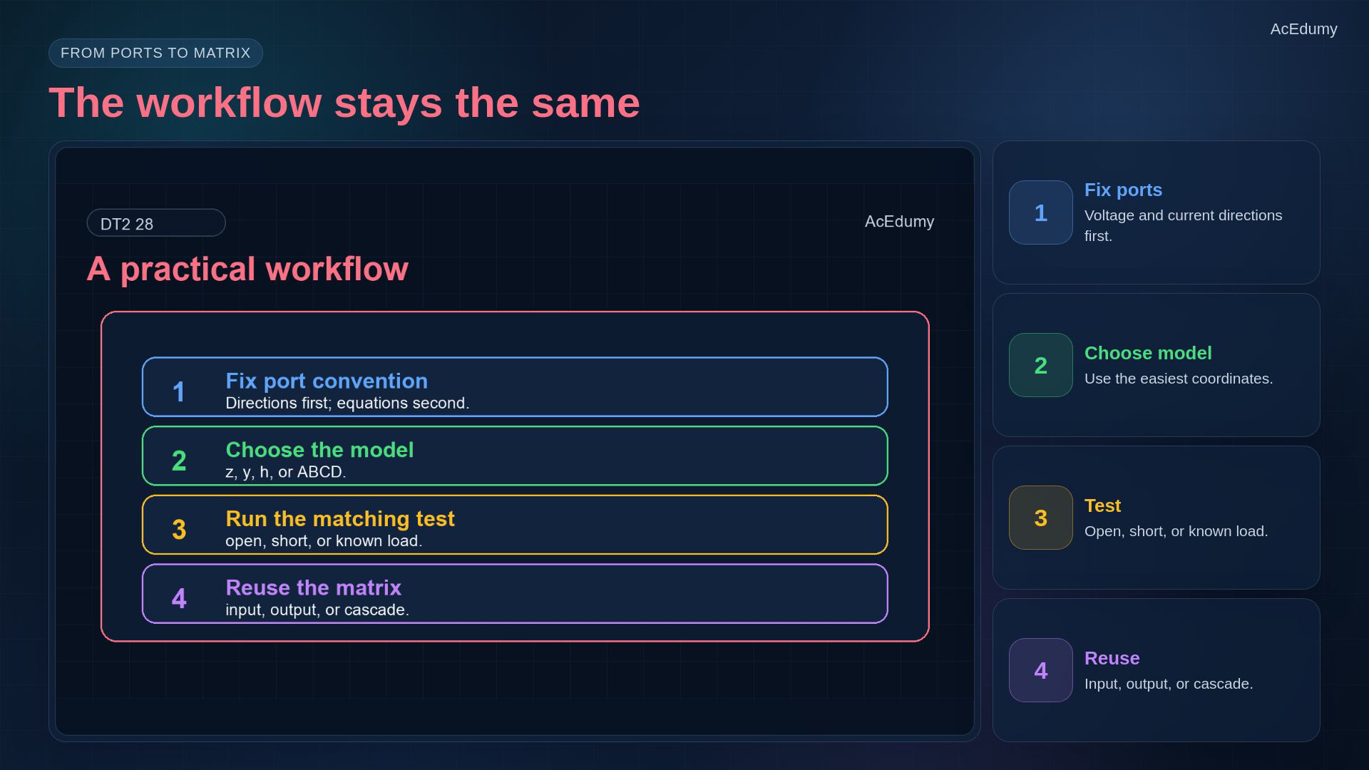
Original-video reference; three diagram roles use reviewed overview or summary frames. Explicit equations, test conditions and port signs are provided in the notebook.
Choose references before equations and preserve them in every conversion.
Fix each voltage polarity and both entering-current references; check how load current is defined.
Check the model exists and that the chosen parameters have the correct units.
Use sufficient independent tests; a single known load does not generally identify all four unknown parameters.
Compute the actual loaded input, output and cascade response; test definitions are not permission to short powered hardware.
Narration transcript
The workflow stays almost the same. First, lock the port convention and the voltage-current directions. Second, choose the parameter set that reduces the calculation. Third, run the matching test: short circuit, open circuit, or known load. Finally, use the matrix to compute input behavior, output behavior, or a cascade product.
9. Summarize mixed variables, cascades and terminations
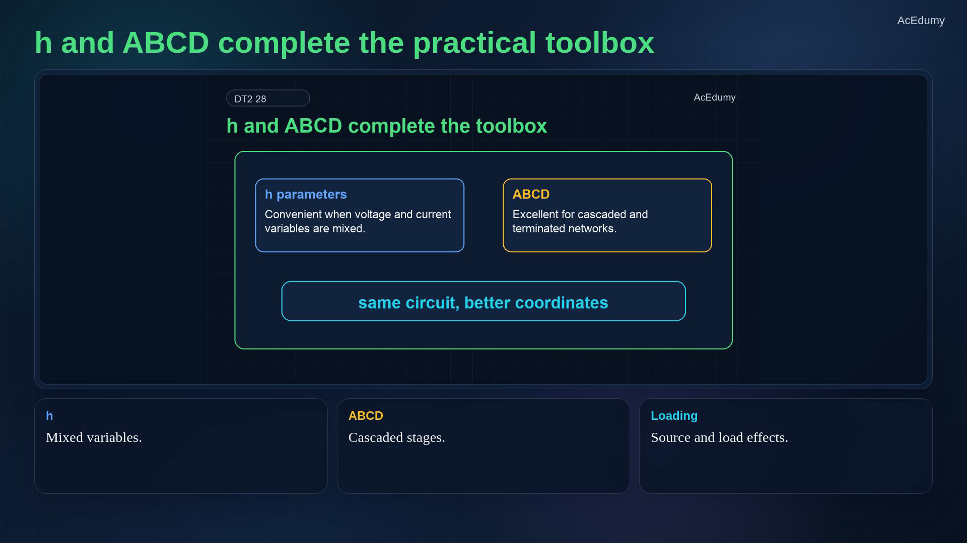
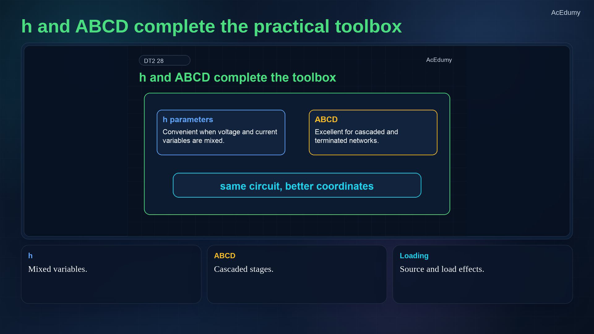
Original-video reference; three diagram roles use reviewed overview or summary frames. Explicit equations, test conditions and port signs are provided in the notebook.
Hybrid and transmission models extend this practical toolbox; they are not every possible two-port representation.
Hybrid form gives input voltage and output current from mixed independent variables.
Transmission form organizes ordered cascades and source/load effects.
Reuse a valid terminal model without forgetting its port conditions, signs, frequency range or linear-operation limits.
Narration transcript
Summary: h parameters and ABCD parameters complete the practical two-port toolbox. h parameters are convenient when voltage and current are mixed. ABCD parameters are excellent for cascaded and terminated networks. The general idea is unchanged: instead of opening the circuit every time, turn it into a useful matrix and reuse it intelligently.