Circuit Theory 1 · Second-Order Transients
#49 Transient Analysis #49 — Underdamped and undamped parallel RLC
Builds the underdamped and undamped natural-response forms from complex roots, connecting envelope, frequency, and energy.
Question
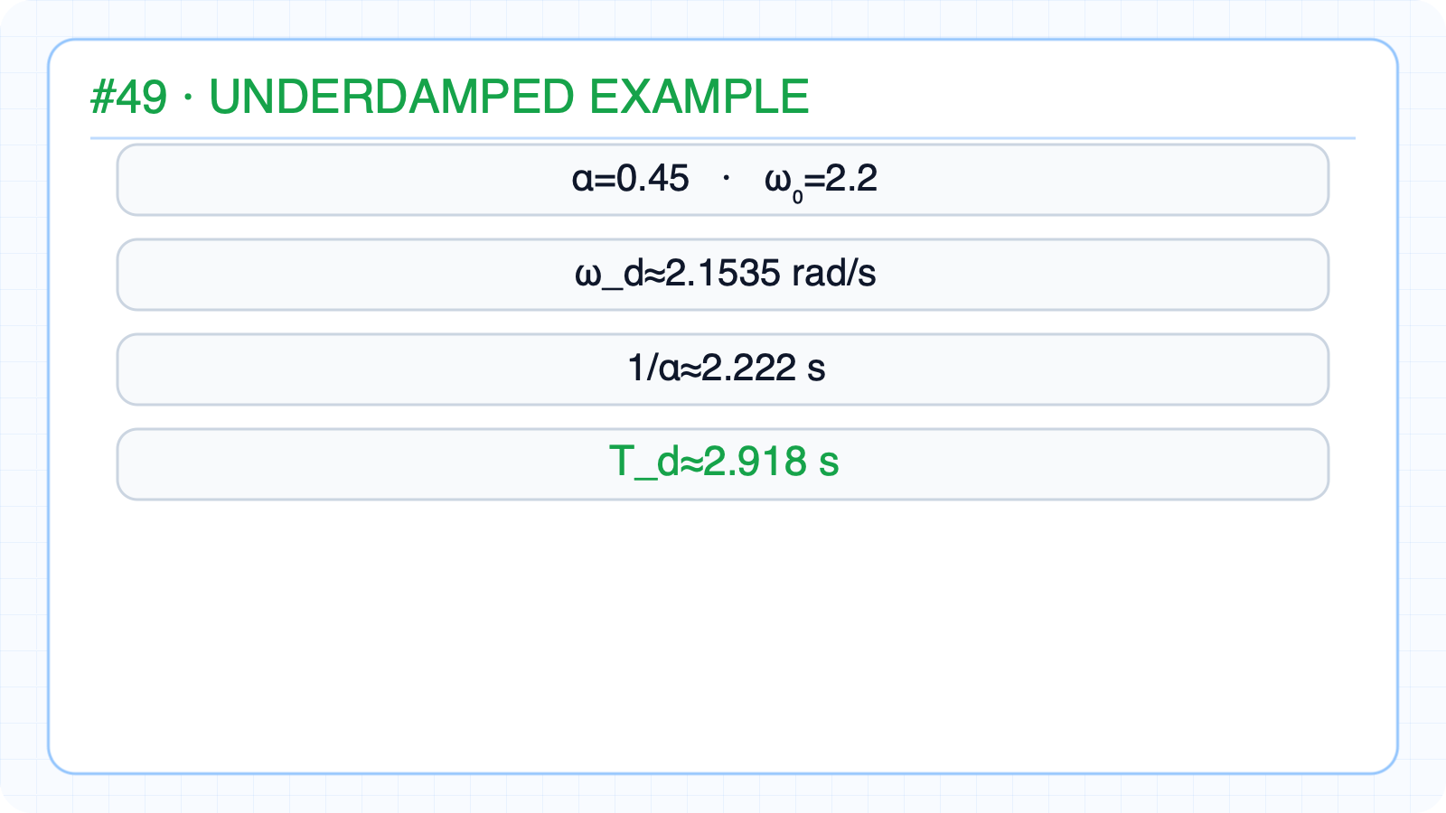
Derive the underdamped and undamped parallel-RLC natural responses; for α=0.45 and ω₀=2.2, calculate ω_d, the envelope constant, and the period.
Written solution and narration transcript(shows the full solution)
Below are all the lines written in the notebook together with the full narration transcript.
1. Separate the two oscillatory cases
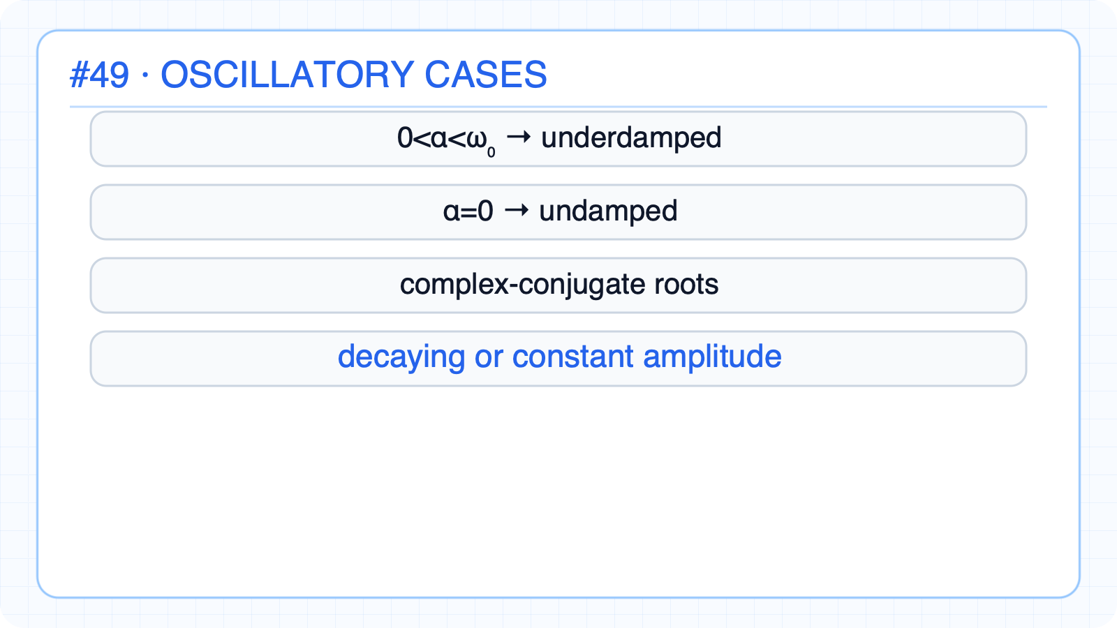
Circuit Theory 1 #49 · Separate the two oscillatory cases The relation between α and ω₀ determines the characteristic roots0<α<ω₀ → underdampedα=0 → undampedBoth cases have complex-conjugate rootsAmplitude decays in the underdamped caseAmplitude remains constant in the undamped caseNarration transcript
In the previous lesson, we covered the non-oscillatory side of second-order response. Now we move to the oscillatory cases. These appear when the roots are no longer two different real numbers. For the parallel R L C circuit, the key question is again the relationship between alpha and omega zero. Today we study the underdamped case and the ideal undamped limit.
2. Underdamped solution form
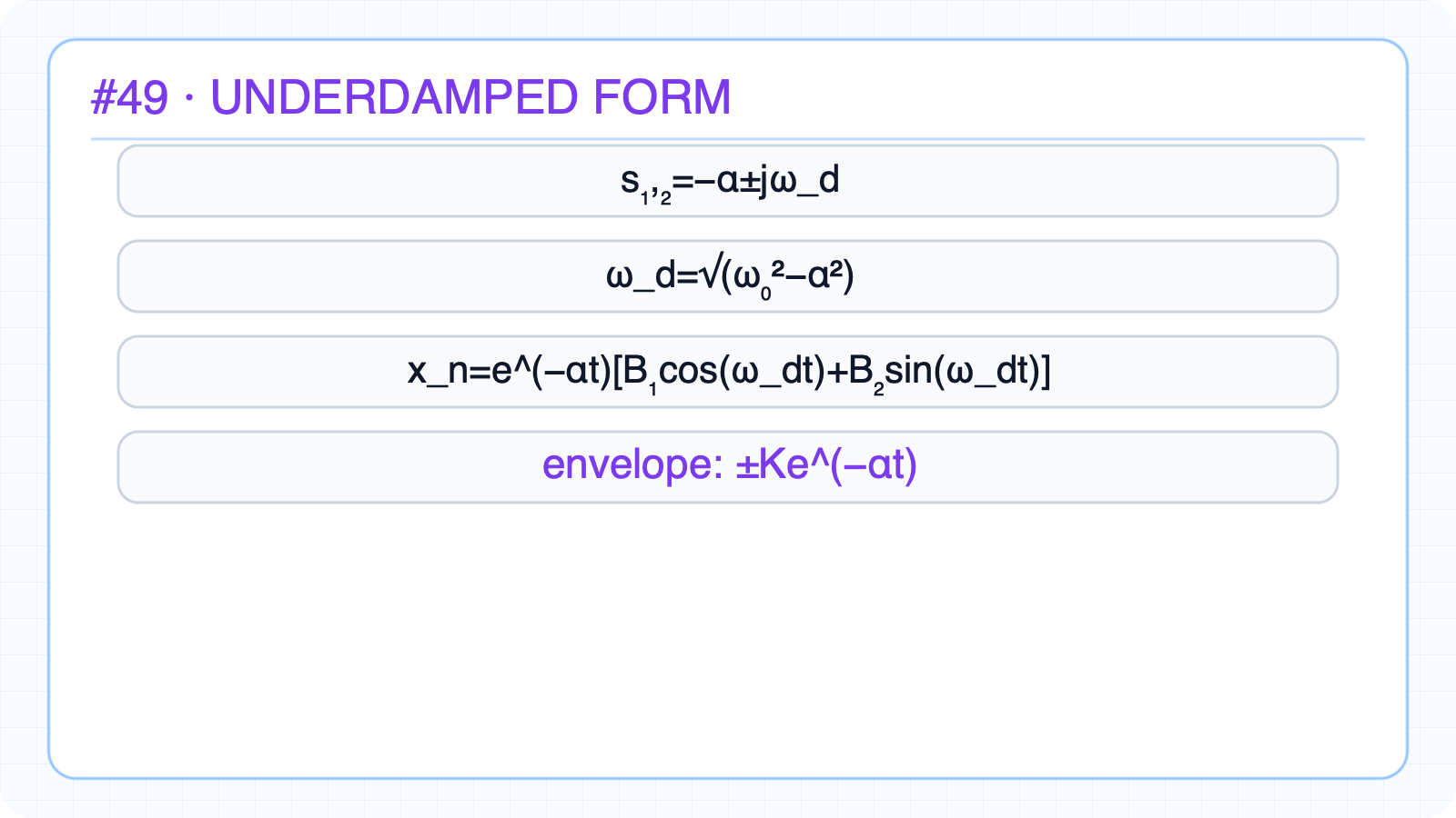
Circuit Theory 1 #49 · Underdamped solution form Condition:ωd is the damped natural angular frequencyThe e−αt envelope shrinks successive peaksOscillation continues while energy falls each cycleNarration transcript
Start with the underdamped case, where alpha is less than omega zero. The characteristic roots become a complex conjugate pair: negative alpha plus or minus j omega d, where omega d equals the square root of omega zero squared minus alpha squared. The natural response therefore takes the form e to the minus alpha t times an oscillating term. In other words, the waveform oscillates, but its amplitude shrinks under an exponential envelope.
3. Underdamped numerical example
Circuit Theory 1 #49 · Underdamped numerical example α=0.45 s⁻¹, ω₀=2.2 rad/sωd=√(2.2²−0.45²)≈2.1535 rad/sEnvelope time constant:Oscillation period:Initial conditions determine B₁ and B₂The decay envelope and oscillation frequency play separate rolesNarration transcript
For example, choose alpha equal to zero point four five and omega zero equal to two point two. Then the response looks like e to the minus alpha t cosine omega d t. The key visual idea is the envelope. The oscillation continues to cross zero, but the peaks get smaller and smaller because energy is dissipated in the resistor. This is the classic damped oscillation shape.
4. Undamped solution form
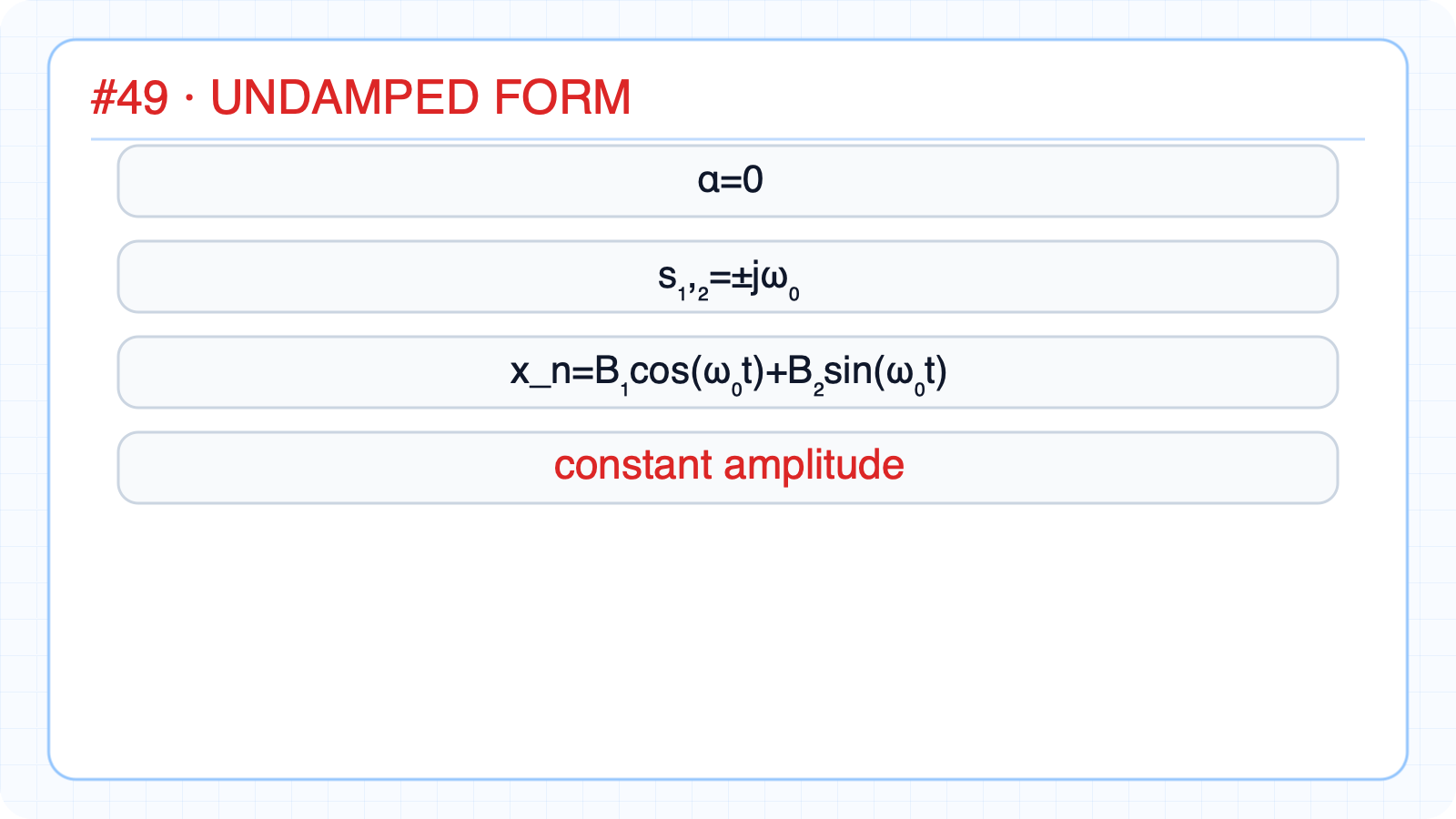
Circuit Theory 1 #49 · Undamped solution form Condition:The exponential envelope becomes e⁰=1The ideal circuit has no resistance or energy lossEnergy moves continuously between L and CAmplitude never decays; oscillation persists at ω₀Narration transcript
Now consider the ideal undamped case. Here alpha equals zero, which means no damping is present. In practice, this is the ideal L C limit. The roots sit exactly on the imaginary axis at plus or minus j omega zero. The natural response becomes a pure sinusoidal combination: B one cosine omega zero t plus B two sine omega zero t. There is no decaying envelope.
5. Compare energy and waveform
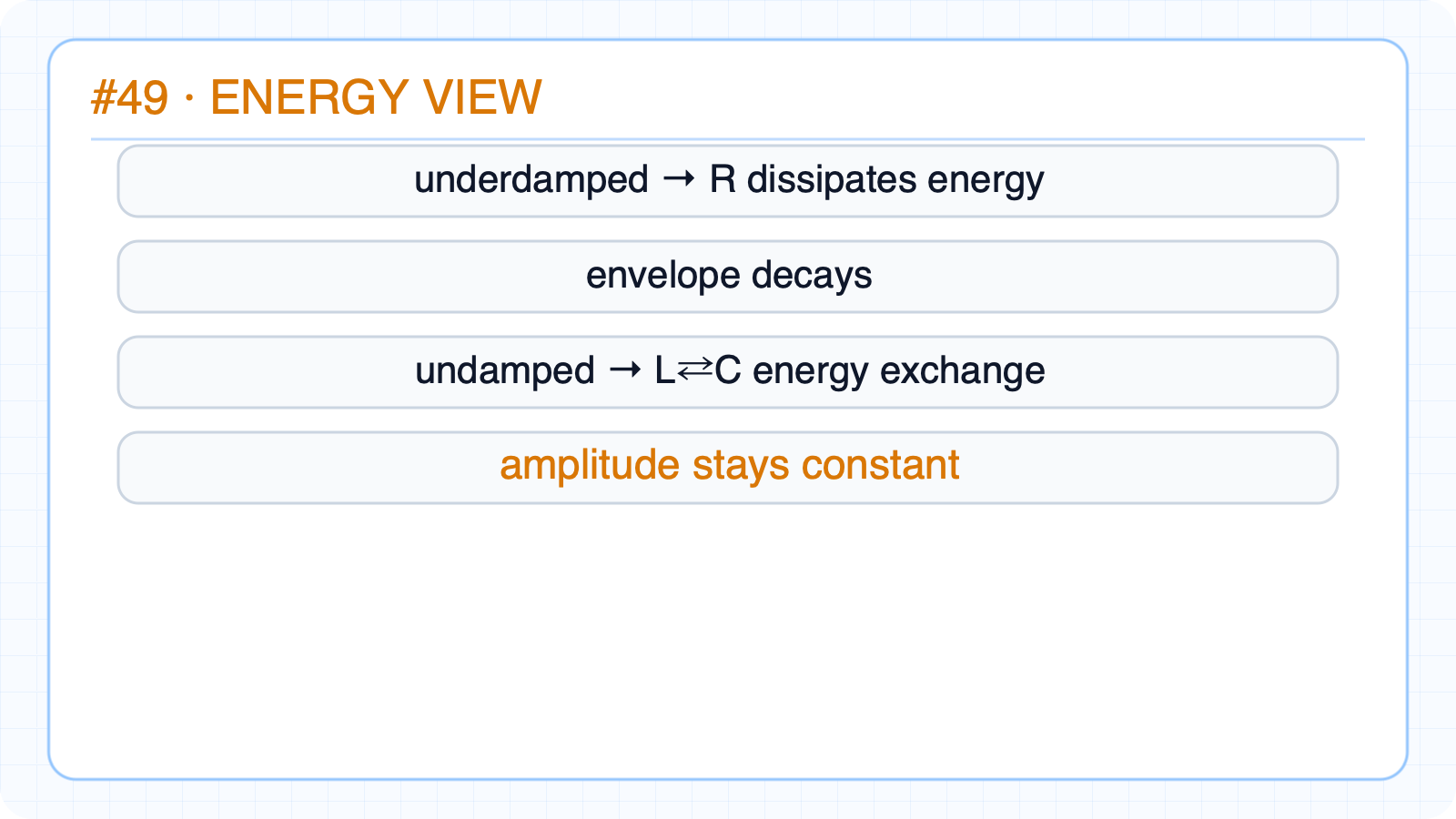
Circuit Theory 1 #49 · Compare energy and waveform Underdamped:R converts stored energy into heatEnvelope: ±Ke−αtThe oscillation frequency ωd is below ω₀Undamped:There is no energy loss and the envelope is constantThe oscillation frequency is exactly ω₀Narration transcript
Compare the two oscillatory cases carefully. In the underdamped response, the circuit still oscillates, but the resistor removes energy over time, so the amplitude decays. In the undamped response, energy keeps exchanging between the capacitor and the inductor without loss, so the amplitude stays constant. Both are oscillatory. The difference is whether the envelope decays or remains flat.
6. Summarize underdamped and undamped response
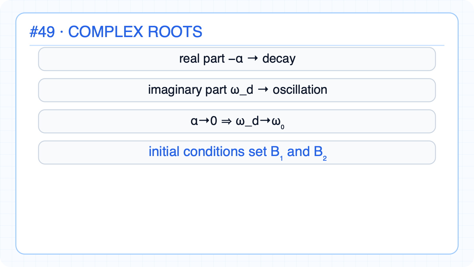
Circuit Theory 1 #49 · Summarize underdamped and undamped response Complex roots create oscillatory responseReal part −α → envelope decay rateImaginary part ωd → oscillation rateAs α approaches zero, ωd approaches ω₀At α=0 the decaying envelope disappearsInitial conditions determine B₁ and B₂Next: combine the natural and forced responsesNarration transcript
Let us summarize. When alpha is less than omega zero, the circuit is underdamped and the roots are complex conjugates. The response oscillates under an exponential envelope, and the damped frequency is omega d. When alpha is zero, the circuit becomes the ideal undamped L C case, with sustained sinusoidal oscillation. Next lesson, we move from natural response cases to the full second-order response with forcing.